Contents
1.1 Some Novel Extensions in DES
1.2 Highlights for the Current Version
1.5.1 Deductive Database Systems
1.5.3 Systems with Formal Relational Query Languages
2.2 Installing and Executing DES
2.2.1.1 Executable Distribution
2.2.2.1 Executable Distribution
2.2.3 Starting DES from a Prolog Interpreter
2.3 The Online Interface DESweb
3.4 Tuple Relational Calculus Mode
3.5 Domain Relational Calculus Mode
4.1.6 Automatic Temporary Views
4.1.12.4 Aggregates and Duplicates
4.1.13 Non-deterministic Functions and Function Predicates
4.1.14 Impure Deterministic Functions and Function Predicates
4.1.16 Relational Division in Datalog
4.1.17 Existential Quantification
4.1.18.1.1 Types on the Intensional Database
4.1.18.1.2 Types on Propositional Relations
4.1.18.2 Nullability (Existence Constraint)
4.1.18.4 Candidate Key (Uniqueness Constraint)
4.1.18.6 Functional Dependency
4.1.18.7 User-defined Integrity Constraints
4.1.20 Limited Domain Predicates
4.1.21.1 Hypothetical Queries and Integrity Constraints
4.1.21.2 Hypothetical Queries and Duplicates
4.1.21.3 Hypothetical Queries and Negation
4.1.22.1 Fuzzy Relations and Approximation Degrees
4.1.22.2 Fuzzy Relations and Properties
4.1.22.3 Weak Unification and Weak Unification Operator
4.1.22.5 Accessing Approximation Degrees
4.1.22.6 An Application: Recommender Systems
4.1.22.7 Fuzzy Restricted Predicates
4.1.22.8 Fuzzy Hypothetical Datalog
4.1.22.9 Fuzzy Datalog Caveats
4.2.4 Data Definition Language
4.2.5 Data Manipulation Language
4.2.6.2 A More Developed SQL Query Description
4.2.6.2.1 TOP, OFFSET, LIMIT and FETCH
4.2.8.7 Automatic Type Casting
4.2.9 (Multi)Set Expressions (Non-Standard)
4.2.9.1 Relational Division in SQL (Non-Standard)
4.2.9.4 Hypothetical SQL Queries (Non-Standard)
4.2.10 Information Schema Language (ISL)
4.2.11 Transaction Management Language (ISL)
4.2.12 SQL Syntax and Semantic Checking
4.2.12.2 SQL Semantic Checking
4.3 (Extended) Relational Algebra
4.5 Domain Relational Calculus
4.7.2 Datalog and Prolog Arithmetic
4.7.3 SQL, TRC and DRC Arithmetic
4.7.5 String Functions and Operators
4.7.6 Date and Time: Data Structures, Functions and Operators
4.7.11 Null-related Predicates
5.1 RDBMS connections via ODBC
5.1.1 Opening an ODBC Connection
5.1.3 Opening Several Connections
5.1.5 Making a Connection the Current One
5.1.7 Schema and Data Visibility
5.1.8 Solving Engine and ODBC Connections
5.1.9 Integrity Constraints, ODBC Connections, and Persistence
5.1.10 Caveats and Limitations
5.1.10.3 Platform-specific Issues
5.2.1 Declaring a Persistent Predicate
5.2.2 Using Persistent Predicates
5.2.3 Processing a Persistence Assertion
5.2.5 Schema of Persistent Predicates
5.2.6 Removing Predicate Persistence
5.2.7 Closing a Persistent Predicate Connection
5.2.8 Schema and Data Visibility
5.2.10.3 Opening and Closing Connections
5.2.10.4 Abolishing Predicates
5.2.10.6 External Database Processing
5.3.3 Safety for Aggregates and Duplicate Elimination
5.3.4 Unsafe Rules from Compilations
5.3.5 Safety for Limited Domain Predicates
5.4 Modes for Unsafe Predicates
5.5.2 Arguments of Built-ins and Metapredicates
5.6 Source-to-Source Transformations
5.10 Datalog Declarative Debugger
5.10.1 Basic Debugging of Datalog Programs
5.10.2 Debugging Datalog Programs with Wrong and Missing Answers
5.10.2.1 TAPI Interface for Datalog Debugging
5.10.2.1.3 Current Question to the User
5.11.2 Missing and Wrong Tuples
5.11.2.3 Displaying Extended Information
5.11.2.4 Automated Benchmarking for Debugging
5.11.2.5 TAPI Interface for SQL Debugging
5.11.2.5.3 Current Question to the User
5.13.2 Logging Script Processing
5.15 System and User Variables
5.17.2 Local and ODBC Databases
5.17.3 Dependency Graph and Stratification
5.17.4 Debugging and Test Case Generation
5.18.1 Notes about the Interface
5.18.4 TAPI-enabled Assertions
5.19 Sandboxing: Enabling Host Safety
5.20 ISO Escape Character Syntax
5.21 Database Instance Generator
5.22 Notes about the Implementation of DES
5.22.3 Dependency Graphs and Stratification: Negation, Outer Joins, and
Aggregates
5.22.4.1 Complete Computations (/optimize_cc)
5.22.4.2 Extensional Predicates (/optimize_ep)
5.22.4.3 Non-recursive Predicates (/optimize_nrp)
5.22.4.4 Stratum (/optimize_st)
5.22.6 Porting to Unsupported Systems
6.1 Relational Operations (files relop.{dl,sql,ra,drc,trc})
6.2 Paths in a Graph (files paths.{dl,sql,ra})
6.3 Shortest Paths (file spaths.{dl,sql,ra})
6.4 Family Tree (files family.{dl,sql,ra})
6.5 Basic Recursion Problem (file recursion.dl)
6.6 Transitive Closure (files tranclosure.{dl,sql,ra})
6.7 Mutual
Recursion (files mutrecursion.{dl,sql,ra})
6.8 Farmer-Wolf-Goat-Cabbage Puzzle (file puzzle.dl)
6.8.1 Dealing with paths (file puzzle1.dl)
6.9 Paradoxes (files russell.{dl,sql,ra})
6.10 Parity (file DLDebugger/parity.dl)
6.11 Grammar (file grammar.dl)
6.12 Fibonacci
(file fib.{dl,sql,ra})
6.13 Hanoi Towers (file hanoi.dl)
9.1 Version Devel of DES (released on January, 13th, 2026)
10................................................................................. Acknowledgements
1. Introduction
The
intersection of databases, logic, and artificial intelligence gave raise to
deductive databases. Deductive database systems are database management systems
built around a logical model of data, and their query languages allow
expressing logical queries. A deductive database system includes procedures for
defining deductive rules which can infer information (in the so-called intensional database) in addition to the
facts loaded in the (so-called extensional)
database. The logic model for deductive databases is closely related to the
relational model and, in particular, with the domain relational calculus. Datalog
is the most known deductive query language (which syntactically is a Prolog subset)
where constructed terms are not allowed as other non-declarative constructs such
as the cut.
Also
following the relational model, relational database systems are well-known and
widespread nowadays. Their formal query languages include relational algebra
and relational calculi but, in practical systems, the de-facto and ANSI/ISO standard SQL is
the language of choice of every relational database vendor. Whilst SQL and
relational formal languages implement a limited form of logic, deductive
database languages implement advanced forms of logic. Database languages are
conceived to be specific-purpose rather than general-purpose languages, and are
targeted at solving database queries. This is contrary to the case of Prolog,
for instance, which is intended as a general-purpose language and its strengths
must not be missed with those of Datalog.[1]
This manual
describes DES, a deductive system which born from the need for teaching Datalog,
and to have a simple, interactive,
multiplatform, and affordable system (not necessarily efficient) for students,
so that they can grasp the fundamental concepts behind a deductive database
with Datalog, Relational Algebra, Tuple Relational Calculus, Domain Relational
Calculus and SQL as query languages. All these query languages do operate over
the same shared database. Pure and extended Datalog are supported. Also, SQL is
supported with a reasonable coverage of the standard for teaching purposes, and
nevertheless with some novel extensions. Supported (extended) relational
algebra includes duplicates, outer joins and recursion. Both relational calculi
and algebra are supported following the syntax of [Diet01]. Original
development of DES was driven by the need for such a tool with features that no
other deductive system (see related work in Section 1.5) enjoyed at the time.
This system is not targeted as a
complete deductive database, so that it does not provide transactions,
security, and other features present in current database systems, but it has grown in different areas.
In particular, it has been added with several additions coming from research
and practical applications. Its web page des.sourceforge.net contains many use cases of this
system in teaching, researching and applications. Statistics also reveal it has
become a widely-used system along time.
As a condensed description, the Datalog Educational System (DES) is a
free, open-source, multiplatform, portable, Prolog-based implementation of a
deductive database system. DES Devel is the current
implementation, which enjoys Datalog, Relational Algebra, Tuple Relational
Calculus, Domain Relational Calculus and SQL query languages, full recursive
evaluation with memoization techniques, full-fledged arithmetic, stratified
negation, duplicates and duplicate elimination, restricted predicates, integrity
constraints, ODBC connections to external relational database management
systems (RDBMSs), Datalog and SQL tracers, a textual API for external
applications, and novel approaches to hypothetical SQL queries and Datalog
rules, declarative debugging of Datalog queries and SQL views, test case generation
for SQL views, modes, null values support, (tabled) outer join, aggregate
predicates, and Fuzzy Datalog. The system is implemented on top of Prolog and
it can be used from a Prolog interpreter running on any OS supported by such interpreter.
Moreover, Windows, Linux and Mac OS X executables are also provided. The
graphical and configurable IDE ACIDE [Saen07] has been specifically
adapted to work with DES. An on-line front-end, DESweb, is also available at https://desweb.fdi.ucm.es.
As being said already, though DES was developed for teaching purposes, it
has been used to develop some novel extensions as introduced next.
1.1
Some
Novel Extensions in DES
A novel contribution implemented in this system is a declarative debugger
of Datalog queries (with several approaches along time [CGS07, CGS08]), which
relies on program semantics rather than on the computation mechanism. The
debugging process is usually started when the user detects an unexpected answer
to a query. By asking questions about the intended semantics, the debugger
looks for incorrect program relations. The initial implementation was
superseded by a recent one [CGS15a] for which more detailed user answers are
allowed. See Section 5.10.
Also, a similar declarative approach has been used to implement an SQL declarative
debugger, following [CGS11b]. There, possible erroneous objects correspond to
views, and the debugger looks for erroneous views asking the user whether the
result of a given view is as expected. In addition, trusted views are supported
to prune the number of questions. This was extended to also include user
information about wrong and missing tuples [CGS12a]. See Section 5.11.
Following the need for catching program errors when handling large
amounts of data, we also include a test case generator for SQL correlated views
[CGS10a]. Our tool can be used to generate positive, negative and both
positive-negative test cases. See Section 0.
Decision support systems usually require assuming that some data are
added to or removed from the current database to make deductions. In this line,
DES introduces Hypothetical Datalog rules [Saen13]
following [Bonn90] (Section 4.1.21).
The novel concept of restricted predicates was introduced to provide support
for negative assumptions in [Saen15] (Section 4.1.19). Hypothetical Datalog has been
extended to the fuzzy setting, which opens new frontiers, such as modifying the
semantics of fuzzy predicates with assumptions and fuzzy equations (Section 4.1.22). Also, limited domain predicates (tightly
related to referential integrity constraints) are a new class of predicates
with a finite meaning and that widen the queries on them, notably with
non-closed negation calls (Section 4.1.20). Also, DES included a novel ASSUME clause for supporting
hypothetical SQL queries and views [DES2.6], which was later changed first to make
temporary relations (common table expressions - CTE) local to their contexts,
and, second, to support negative assumptions in [DES3.7] (Section 4.2.9.4). For positive assumptions, ASSUME statements
can be alternatively specified with a WITH clause with
minor changes. Both are compiled into hypothetical Datalog rules. This makes a WITH encapsulation
something natural in the realms of hypothetical Datalog.
For dealing with vagueness and imprecise information, Fuzzy logic
programming has been applied to develop a fuzzy deductive database following
[JS10] (Section 4.1.22), with Fuzzy Datalog as its query language.
Since this system is targeted mainly towards teaching, we have provided
an SQL semantic checker [Saen19] that raises warnings for, though syntactically
correct SQL statements, possible incorrect ones, following the descriptions in
[BG06]. Some errors include inconsistent conditions, lack of correlations in
joins, unused tuple variables and the like. In the same line, an optimizing SQL
compiler generates Datalog rules which are translated back into SQL. If the
optimized SQL query is better than the original one, it is displayed as a
better alternative. This helps students to check their queries for unnecessary
constructs and develop neater formulations.
1.2
Highlights
for the Current Version
This version introduces several upgrades, mainly
driven by teaching needs. First, when submitting an SQL query (top-level, with
create view...) the system may display a better formulation if one is found.
This process involves compiling the query into Datalog rules, applying
optimizations, and then compiling the resulting rules back into SQL. If the
optimized query has fewer nodes in its syntactic tree than the original or, if
it is more efficient (e.g., by using WHERE instead
of HAVING conditions) then it
is suggested as a hint for a better alternative. Second, as a collateral effect
of the improved Datalog to SQL compilation (which now handles more built-ins) a
wider set of rules in persistent predicates can be externally stored as SQL
views. Third, both SQL and RA languages have extended coverage, including SQL ALTER
TABLE, UPDATE and SELECT statements,
and well as additional RA set operations. Fourth, improved SQL translations for
AR, DRC and TRC are now available. Finally, DES includes various enhancements,
new commands, and refinements. Section 9.1 includes the complete list of
enhancements, changes and bug fixes.
1.3 Features of DES in Short
·
Free,
multiplatform, portable, and open-source.
It can be used in any OS platform (Windows,
Mac, Linux, ...), running on one of the supported Prolog interpreters. Moreover,
portable executable applications are provided for Windows, Mac, and Linux.
·
Interactive.
Based on a command line interpreter, you can
play with DES by submitting queries, modifying the database, and processing
commands.
·
Five
query languages and one shared database.
Datalog, SQL, Relational Algebra (RA), Tuple
Relational Calculus (TRC), Domain Relational Calculus (DRC) and with access to
the same database, either locally or externally stored (via ODBC
connections and/or persistent predicates). Examine the equivalent Datalog code
resulting from compiling other languages (/show_compilations on).
·
Fuzzy
Datalog:
Formal concepts supporting the fuzzy logic
programming system Bousi~Prolog are translated into the deductive database
system. Hypothetical fuzzy reasoning has been also added.
·
Graphical
user interface.
The Java-based ACIDE graphical environment
(screenshot) has been configured for a specific connection to DES via the
textual application programming interface (TAPI). It enjoys Datalog, SQL, RA,
TRC, and DRC syntax highlighting, command buttons and interactive console,
therefore easing its use by decreasing the number of keystrokes. In addition,
an Emacs environment can be used.
·
Online
graphical user interface.
An online front-end DESweb is available at https://desweb.fdi.ucm.es, which can be used to try DES
without installing it. Though it has many less features than the desktop Java
front-end, it suffices for many needs in introductory courses.
·
Database
updates.
The database can be modified with both SQL DML
and system commands.
·
Null
values and outer joins for three languages: Datalog, RA and SQL.
·
Aggregates.
Typical aggregates as count, sum, min, max, avg, and times for SQL, RA and Datalog are
included. Datalog aggregates include both aggregate predicates and aggregate
functions (to be used in expressions). Grouping is supported and groups built on-the-fly
with Datalog auto-grouping.
·
Multisets.
Duplicates can be enabled or disabled in
Datalog, RA and SQL processing. Discard duplicates with distinct operators.
·
Hypothetical
queries, views and rules in both Datalog and SQL.
Use the implication => in Datalog to build “what-if”
applications in a business intelligence scenario. Use the novel ASSUME SQL clause to build hypothetical
queries and views.
·
Relational
database access via ODBC.
ODBC sources of data can be seamlessly
accessed. Connect DES to any DBMS supporting such connections (MySQL, MS
Access, Oracle, ...)
·
Persistency.
Predicates and relations can persist on
external data sources via ODBC connections. Examine the SQL statements sent to
the external database for persistent predicates (/show_sql on) .
·
Modes.
An input mode warns users about the need to
ground an argument in queries for an unsafe predicate.
·
Highly
configurable system on-the-fly.
Multiple features can be turned on and off and
parameterized via commands.
·
Stratified
negation.
·
Novel
and extended SQL features include:
o
Enforcement
of functional dependencies.
o
Hypothetical
queries and views.
o
DIVISION relational operation.
o
Mutual
and non-linear recursion
·
Integrity
constraints.
o
Domain.
o
Types.
o
Primary
key.
o
Referential
integrity.
o
Functional
dependency.
o
Check
constraints (user-defined).
o
...
and several typical others.
Constraint checking can be enabled or disabled.
·
Declarative
debugging for Datalog and SQL.
Several declarative debuggers have been
included along time in DES with the aim to debug towards intended semantics rather
than procedural semantics. In addition, debugging can be used with existing external
databases such as DB2, MySQL, PostgreSQL and Oracle.
·
Test
case generation for SQL views.
This prototype can be used for working with
views over large tables and test them with the test cases, instead of with the
actual tables.
·
SQL
database generator.
If you need SQL database instances for your
benchmarks, generate them randomly at will.
·
Full-fledged
arithmetic.
Write arithmetical expressions with a wide set
of arithmetical functions, operators and constants. Unlimited precision integer
arithmetic is provided thanks to the underlying Prolog systems.
·
Type
system for Datalog, RA, TRC, DRC and SQL.
Whilst SQL require typed relations, Datalog
predicates can be optionally typed to feeling the benefits of typed relations
and type inference. Automatic type casting à
la SQL in both settings can be enabled with the command /type_casting on. Explicit type casting is allowed
with both an SQL function and a Datalog predicate.
·
Syntax
checking for all languages with informative error messages, and SQL semantic
checking with informative warning messages.
·
Connecting
DES to the outside programmatic world.
DES can be plugged to a host system via
standard streams using the textual application interface TAPI. DES can be
connected to any development system supporting standard stream operations:
Java, C++, VB, Python, Lua, ... Alternatively, use the underlying Prolog API's
to generate executables or run-time systems with access to several languages
(Java, C++, ...).
·
Configurable
look and feel.
o
Pretty-printers
for Datalog, RA and SQL.
o
Single
and multiline modes.
o
Compact
or separated display lines.
·
Batch
execution.
o
Provide
a file with DES inputs and log the results into another file. Several logs at a
time are supported.
o
Use
batch commands and system variables for execution control.
·
Implementation
includes:
o
Source-to-source program transformations:
§ Safety. Safety transformations can
be enabled to deal with some unsafe rules. Also, unsafe rules can be used to
experiment in conjunction with modes.
§ Built-ins. Programs with outer join
calls are transformed in order to be computed by the underlying tabled,
fixpoint method.
o
Tabling. Answer tables are used for implementing
fixpoint and caching computations.
·
Development
mode.
This mode, when enabled, helps to understand
how the system works (/development on). Transformed and compiled programs can be examined.
1.4 Future Enhancements
The
following list (in order of importance) suggests some points to address for
enhancing DES:
·
Disjunctive
heads
·
Information
about cycles involving negation in the loaded program
·
Complete
algorithm for finding undefined information
·
Constraints
à la CLP (real, integer, enumerated types, strings)
·
Faster
parsers
If you find
worthwhile for your application either some of the points above, or others not
listed, please inform the author for trying to guide the implementation to the
most demanded points.
1.5 Related Work
Origins of
deductive databases can be found in automatic theorem proving and, later, in
logic programming. Minker [Mink87] suggested that Green and Raphael [GR68] were
the pioneers in discovering the relation between theorem proving and deduction
in databases. They developed several question–answer systems using a version of
the Robinson resolution principle [Robi65], showing that deduction can be
systematically performed in a database environment. Other pioneer systems were
MRPPS [MN82], DEDUCE–2 [Chan78] and DADM [KT81]. See Section 1.5 for references to other current
deductive database systems.
There has
been a high amount of work around deductive databases [RU95] (its interest
delivered many workshops and conferences for this subject) which dealt to
several systems. However, to the best of our knowledge, there is no a friendly
system oriented to introducing deductive databases with several query languages
to students. Nevertheless, on the one hand, we can comment some representative
deductive database systems, and, on the other hand, some technological
transfers to face real-world problems. Finally, we comment on existing systems
with formal relational query languages.
1.5.1 Deductive Database Systems
This
section collects and describes some deductive database systems developed so
far:
·
Logica
(https://logica.dev) is an open‑source declarative language built on Datalog, designed to simplify
complex queries and reasoning over data. Released in 2021 as a successor to
Yedalog, it integrates with BigQuery and offers a more expressive, Prolog‑like syntax for writing recursive rules, logical constraints, and
aggregations. Its goal is to make data analysis more concise and readable than
SQL, while retaining the power of logical programming for advanced use cases in
teaching, research, and large‑scale data processing.
·
Mangle
(https://github.com/google/mangle)
is an open‑source deductive programming
language built on Datalog, designed to handle fragmented and complex data
across modern systems. Implemented as a Go library, it extends traditional
logic programming with support for aggregations, external functions, and
optional typing, making it suitable for large‑scale data analysis, dependency tracking, and security applications.
·
4QL
[MS11] (http://4ql.org) is a recent
development of a rule-based database query language with negation allowed in
bodies and heads of rules, which is founded on a four-valued semantics with
truth values: true, false, inconsistent and unknown. It provides means for a
uniform treatment of Open and Local Closed World, other nonmonotonic/commonsense
formalisms, including various variants of default reasoning, autoepistemic
reasoning and other formalisms application-specific disambiguation of
inconsistent information, including defeasible reasoning.
·
Logic
Query Language (LogiQL, http://www.logicblox.com/technology.html)
is a declarative programming language derived from Datalog and developed by
LogicBlox Inc. for their LogicBlox database engine. It has been designed
including advanced techniques for query evaluation, concurrency management,
network optimization, program analysis, declarative and reactive programming
models.
·
QL
(https://semmle.com/ql) from Semmle is an
object oriented Datalog-based language for read-only databases.
·
ConceptBase
[JJNS98] (http://conceptbase.sourceforge.net/)
is a multi-user deductive object manager mainly intended for conceptual modelling
and coordination in design environments. It is multiplatform, object-oriented,
it enjoys integrity constraints, database updates and several other interesting
features.
·
The
LDL project at MCC lead to the LDL++ system [AOTWZ03], a deductive database
system with features such as X-Y stratification, set and complex terms,
database updates and aggregates. It has been replaced by DeAL. The Deductive
Application Language (DeAL) System (http://wis.cs.ucla.edu/deals/)
is a next-generation Datalog system. The objective of the DeALS project is to
extend the power of Datalog with advanced constructs with strong theoretical
foundations. DeAL supports stratified aggregation, negation and
XY-stratification. DeAL also supports new monotonic aggregates that can be used
in recursive rules.
·
DLV
[FP96] (http://www.dlvsystem.com/dlv/)
is a multiplatform system for disjunctive Datalog with constraints, true
negation (à
·
XSB
[RSSWF97] (http://xsb.sourceforge.net/)
is an extended Prolog system that can be used for deductive database
applications. It enjoys a well–founded semantics for rules with negative
literals in rule bodies and implements tabling mechanisms. It runs both on
Unix/Linux and Windows operating systems. Datalog++ [Tang99] is a front-end for
the XSB system.
·
bddbddb
[WL04] (http://bddbddb.sourceforge.net/)
stands for BDD-Based Deductive DataBase. It is an implementation of Datalog
that represents the relations using binary decision diagrams (BDD's). BDD's are
a data structure that can efficiently represent large relations and provide
efficient set operations. This allows bddbddb to efficiently represent and
operate on extremely large relations.
·
IRIS
(Integrated Rule Inference System) [IRIS2008] is a Java implementation of an
extensible reasoning engine for expressive rule-based languages provided as an
API. Supports safe or un-safe Datalog with (locally) stratified or well-founded
negation as failure, function symbols and bottom-up rule evaluation.
·
Coral
[RSSS94] is a deductive system with a declarative query language that supports
general Horn clauses augmented with complex terms, set–grouping, aggregation,
negation, and relations with tuples that contain (universally quantified)
variables. It only runs under Unix platforms. There is also a version which
allows object–oriented features, called Coral++ [SRSS93].
·
FLORID
(F-LOgic Reasoning In Databases) [KLW95] is a deductive object-oriented
database system supporting F-Logic as data definition and query language. With
the increasing interest in semistructured data, Florid has been extended for
handling semistructured data in the context of Information Integration from the
Semantic Web.
·
The
NAIL! project delivered a prototype with stratified negation, well–founded
negation, and modularity stratified negation. Later, it added the language
Glue, which is essentially single logical rules, with SQL statements wrapped in
an imperative conventional language [PDR91, DMP93]. The approach of combining
two languages is similar to the aforementioned Coral, which uses C++. It does
not run on Windows platforms.
·
Another
deductive database following this combination of declarative and imperative
languages is Rock&Roll [BPFWD94].
·
ADITI
2 [VRK+91] is the last version of a deductive database system which uses the
logic/functional programming language Mercury. It does not run on Windows
platforms. There is no further development planned for Aditi.
See also
the Datalog entry in Wikipedia (http://en.wikipedia.org/wiki/
Datalog).
1.5.2 Technological Transfers
Datalog has
been extensively studied and is gaining a renowned interest thanks to their
application to ontologies [FHH04], semantic web [CGL09], social networks
[RS09], policy languages [BFG07], and even for optimization [GTZ05]. Companies
as LogicBlox, Exeura, Semmle, DLVSYSTEM s.r.l. and Lixto embody Datalog-based
deductive database technologies in the solutions they develop. The high-level
expressivity of Datalog and its extensions has therefore been acknowledged as a
powerful feature to deal with knowledge-based information.
The first
commercial oriented deductive database system was the Smart Data System (SDS)
and its declarative query language Declarative Reasoning (DECLARE) [KSSD94], with support for stratified negation and sets.
Currently, XSB and DLV have been projected to spin-off companies and they
develop deductive solutions to real-world problems.
1.5.3 Systems with Formal Relational Query Languages
Several
implementations of formal relational query languages exist. One of the most
known is WinRDBI (https://winrdbi.asu.edu/),
a system including SQL, RA, and tuple and domain relational calculi (TRC and
DRC, respectively). It includes a GUI and allows the definition of views in
each language. This system is described in the book [Diet01] as a tool for
learning formal languages. Another system is RAT (http://www.slinfo.una.ac.cr/rat/rat.html)
which allows students to write statements in RA which are translated to SQL in
order to verify the correct syntax for these expressions. RAT also allows connections
to relational databases. Also, Chris Date and Hugh Darwen proposed a language
called Tutorial D intended for use in teaching relational database theory, and
its query language also draws on ISBL's ideas. Rel (http://reldb.org/)
is an implementation of Tutorial D as a true relational database management
system. LEAP (http://leap.sourceforge.net)
is a relational database management system developed at the Oxford Brookes
University (UK) which includes pure relational algebra. Relational Algebra
System for Oracle and Microsoft SQL Server (http://www.cse.fau.edu/~marty/),
developed by M.K. Solomon at the Florida Atlantic University (USA), features
relational algebra with division operating on those existing RDBMS's.
2. Installation
This
section explains how to download the available distributions (binary, sources,
bundle with the graphical environment ACIDE), their contents, and hints for
installations and configurations. If you do not want to install the system, you
can use it via the online interface as explained in Section 2.3.
2.1 Downloading DES
You can
download the system from the DES web page via the URL:
http://des.sourceforge.net/
There, you can find source distributions for several Prolog interpreters
and operating systems, and executable distributions for MS Windows, Linux and
Mac OS X.
2.1.1 Source Distribution
Under the source distribution, there are several versions depending on
the Prolog interpreter you select to run DES: either SICStus Prolog [SICStus] or SWI-Prolog [SWI]. However,
adapting the code in the file des_glue.pl, it could be ported to any other Prolog system. (See
Section 5.22.3 for porting to unsupported systems.) We have
tested DES under SICStus Prolog 4.4.1 and SWI–Prolog 7.6.4), and several operating systems (MS Windows XP/Vista/7/8/10,
Ubuntu 10.04/12.04/16.04/18.04, and Mac OS X Snow Leopard/Sierra/High Sierra/El
Capitán).
The source distribution comes in a single archive file containing the
following:
· readmeDES<version>.txt. A quick
installation guide and file release contents.
· des.pl. Core of DES, including Datalog processor.
· des_atts.pl. Attributed variables of
the host Prolog system.
· des_commands.pl. System commands.
· des_common.pl. Common predicates to
different files.
· des_dbigen.pl. SQL database
instance random generator.
· des_dcg.pl. DCG
expansion.
· des_dl_debug.pl. Datalog declarative
debuggers.
· des_drc.pl. DRC processor.
· des_fuzzy.pl. Fuzzy Datalog
subsystem.
· des_glue.pl. Contains particular
code for the selected host Prolog system.
· des_help.pl. Help system.
· des_ini.pl. Initialization files.
· des_modes.pl. Modes for Datalog
predicates and rules
· debug/des_pchr.pl. CHR program for
debugging Datalog predicates
· des_persistence.pl. Persistence
for Datalog predicates
· des_ra.pl. RA processor
· des_sql.pl. SQL
processor
· des_sql_semantic.pl. SQL semantic checker
· des_sql_debug.pl. SQL
declarative debugger
· des_tc.pl. Test case generator for
SQL views
· des_trace.pl. Tracers for SQL and
Datalog
· des_trc.pl. TRC processor
· des_types.pl. Type inferrer and
checker for SQL, RA and Datalog
· doc/manualDESDevel.pdf. This manual
· doc/release_notes_history_DES.pdf. Releases
notes history of previous versions
· examples/* Example files, some of
them discussed in Section 6
· license/* A verbatim copy of the GNU Lesser General Public License for this distribution
· readmeDESDevel.txt. A quick installation guide and release notes
2.1.2 Executable Distribution
2.1.2.1 Windows
From the same URL above, you can download a Windows executable
distribution in a single archive file containing the following:
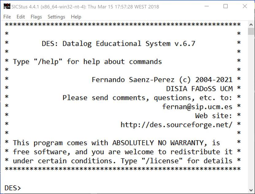
· des.exe. Console executable file,
intended to be started from a OS command shell, as depicted in the next figure:
· deswin.exe. Windows-application executable
file, as depicted below:
Please note that the menu bar above is inherited
from the host Prolog system and all its settings apply to such system, not to
DES. However, there are some menu items that can be useful.
For the SICStus executable:
o
File
® Save
Transcript: Save the current window buffer to a file.
o
Edit:
For clipboard operations. "Automatic Copy" means that by selecting
text, it will automatically copied to the clipboard.
o
Keyboard
shortcuts for clipboard are: Ctrl+Insert (Copy), and Shift+Insert (Paste)
o
Settings
® Window
Settings ® save lines: Number of lines in the window
buffer.
o
Settings
® Fonts:
Select font and size
o
Settings
® Save
Settings: Save current settings for the next session.
For the SWI-Prolog executable:
o
Edit:
For clipboard operations. Automatic copy is always enabled.
o
Keyboard
shortcuts for clipboard are: Ctrl+C (Copy), and Ctrl+V (Paste)
o
Settings
® Fonts:
Select font and size
· *.dll. DLL libraries for the runtime system
·
doc/manualDESDevel.pdf. This manual
·
doc/release_notes_history_DES.pdf. Releases
notes history of previous versions
·
examples/*.dl. Example
files which will be discussed in Section 6
· license/*. A verbatim copy of the GNU Lesser General Public License for this distribution
· readmeDESDevel.txt. A quick installation guide and release notes
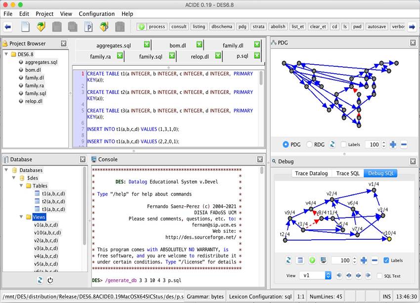
2.1.2.2 DES+ACIDE Bundle
From the same URL above, you can download a bundle including both DES and
the integrated development environment ACIDE, preconfigured to work with DES,
and including the configuration file des.cnf for DES. The following figure is a snapshot of the
system taken in a Windows 10 64 bit system:
2.1.2.3 Linux
From the same URL above, you can download a Linux executable distribution
in a single archive file containing the following:
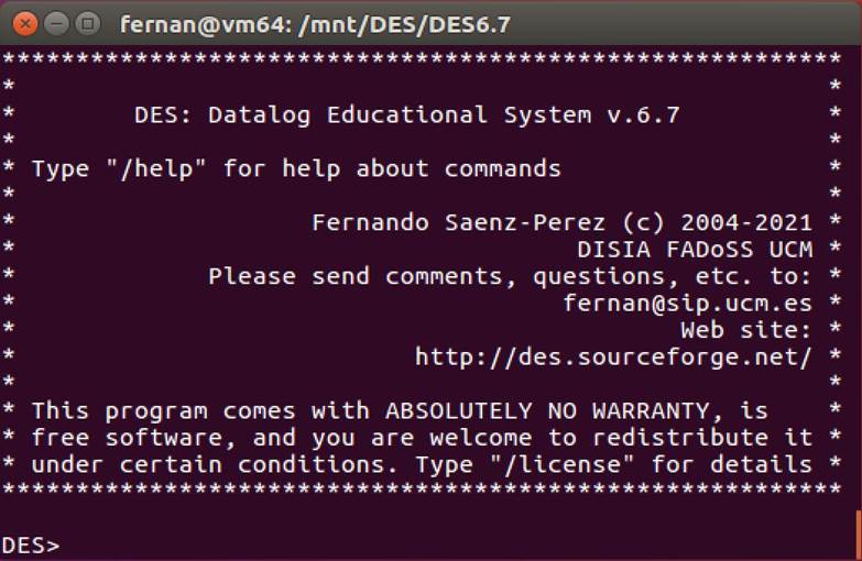
· des. Console
executable file
· doc/manualDESDevel.pdf. This manual
· doc/release_notes_history_DES.pdf. Releases
notes history of previous versions
· examples/*. Example files which
will be discussed in Section 6
· license/*. A verbatim copy of the GNU Lesser General Public License for this distribution
· readmeDESDevel.txt. A quick installation guide and release notes
The following screenshot has been taken in Ubuntu 16.04 LTS 64bit:
An ACIDE bundle can be downloaded for Linux and
including the configuration file des.cnf for DES. The following snapshot shows this running on
Ubuntu 18.04 LTS 64bit:
2.1.2.4 Mac OS X
From the same URL above, you can download a Mac OS X executable
distribution in a single archive file containing the following:
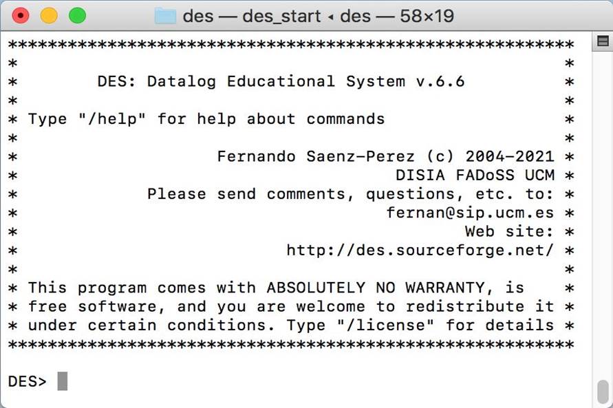
· des. Console
executable file
· doc/manualDESDevel.pdf. This manual
· doc/release_notes_history_DES.pdf. Releases
notes history of previous versions
· examples/*. Example files which
will be discussed in Section 6
· license/*. A verbatim copy of the GNU Lesser General Public License for this distribution
· readmeDESDevel.txt. A quick installation guide and release notes
The following screenshot has
been taken in Mac OS X High Sierra:
There is also an ACIDE bundle that can be downloaded for Mac OS X and
including the configuration file des.cnf for DES. The following snapshot shows this running on
Mac OS X High Sierra:
2.1.3 Other Interfaces
Other interfaces include Emacs and Crimson Editor.
2.1.3.1 Emacs
The first one is a contribution of Markus Triska and provides an
integration of DES into Emacs. Once a Datalog file has been opened, you can
consult it by pressing F1 and submit
queries and commands from Emacs. This
works at least in combination with SWI Prolog
(it depends on the -s switch);
other systems may require slight
modifications. For its installation, copy des.el (as found in the contributions web page)
to your home directory and add to your .emacs:
(load "~/des")
; adapt the following path as necessary:
(setq des-prolog-file "~/des/systems/swi/des.pl")
(add-to-list 'auto-mode-alist
'("\\.dl$" . des-mode))
Restart Emacs, open an *.dl file to load
it into a DES process (this currently only works with SWI-Prolog). If the
region is active, F1 consults
the text in the region. You can then
interact with DES as on a terminal. Next figure shows DES running on Emacs:
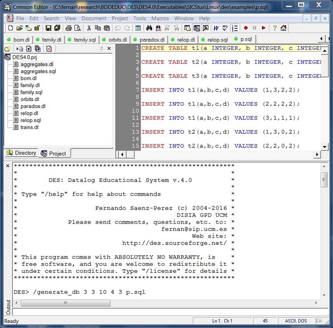
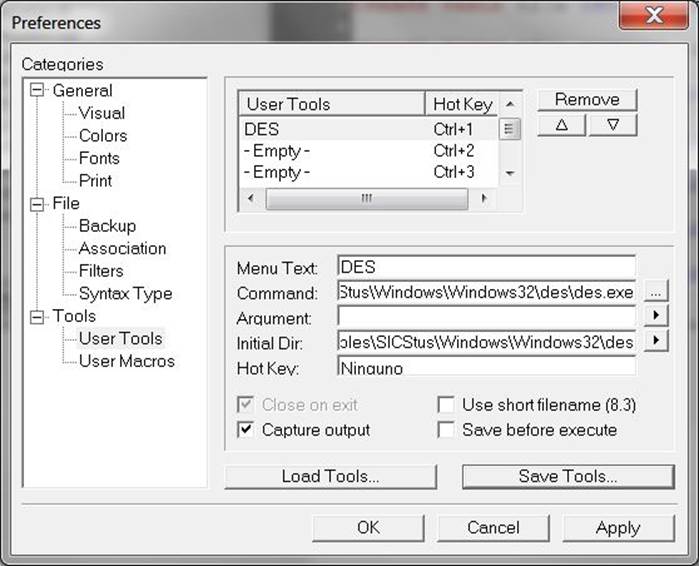
2.1.3.2 Crimson Editor 3.70
The second interface run on Windows and is obtained by configuring
Crimson Editor 3.70 to work with DES as an external tool whose output is
captured by Crimson and input can be sent to DES. In Tools->Conf. User Tools, fill in the Preferences dialog box the path to
the console executable in the Command input box.
Other alternative is to start a Prolog system with an initial goal, as
described in Section 2.2.1.2.
Then, in this case, pressing Ctrl+1 starts the DES console:
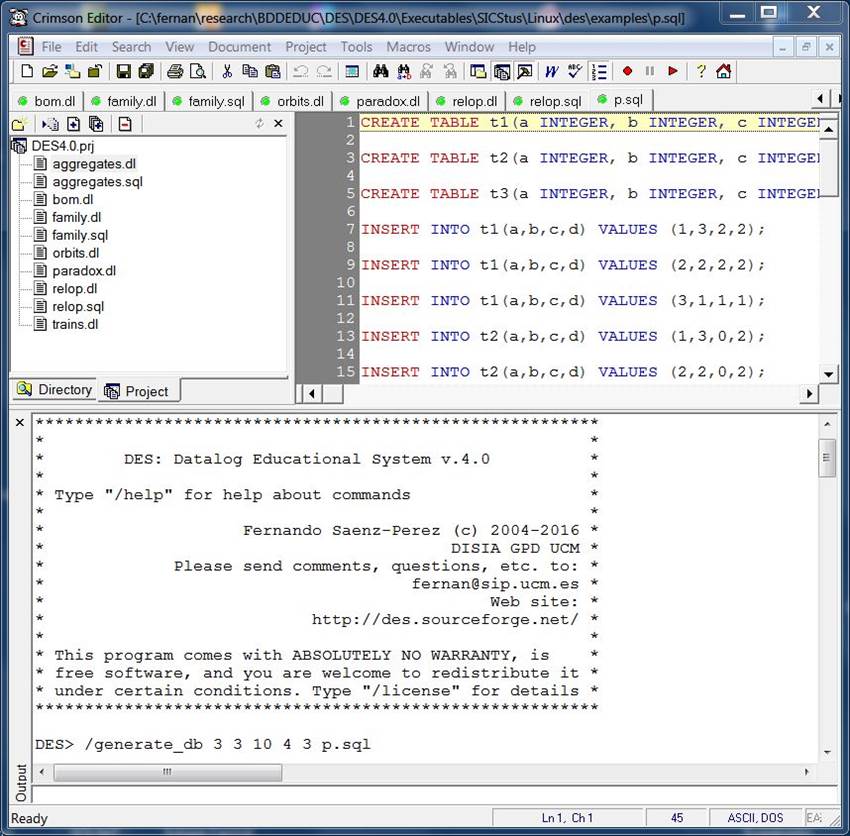
Crimson Editor also lets you to play with multiple editors, syntax
highlighting, projects, and several useful tools. The input can be typed in the
input box below or by clicking with the secondary mouse button to select Input.
2.2 Installing and Executing DES
Unpack the distribution archive file into the
directory you want to install DES, which will be referred to as the
distribution directory from now on. This allows you to run the system, whether
you have a Prolog interpreter or not (in this latter case, you have to run the
system either on MS Windows, Linux or Mac OS X).
Although there is no need for further setup and
you can go directly to Section 2.2.3, you can also configure a more user-friendly way for
system start. In this way, you can follow two routes depending on the operating
system.
2.2.1 MS Windows
2.2.1.1 Executable Distribution
Simply create
a shortcut in the desktop for executing the executable of your choice: either des.exe, or deswin.exe
or des_acide.jar. The former is a console-based
executable, the second is a windows-based executable, and the latter is a Java
application that includes a call to the binary des.exe. Executables
have been generated with SICStus Prolog and SWI-Prolog, so that all notes relating
these systems in the rest of this document also apply to these executables. In
addition, since it is a portable application, it needs to be started from its
distribution directory, which means that the start-up directory of the shortcut
must be the distribution directory.
2.2.1.2 Source Distribution
Perform the
following steps:
1.
Create
a shortcut in the desktop for running the Prolog interpreter of your choice.
2.
Modify
the start directory in the “Properties” dialog box of the shortcut to the
installation directory for DES. This allows the system to consult the needed
files at startup.
3.
Append
the following options to the Prolog executable path, depending on the Prolog
interpreter you use:
(a)
SICStus
Prolog: -l des.pl
(b)
SWI-Prolog:
-g "ensure_loaded(des)" (remove --win_app if present)
Another
alternative is to write a batch file similar to the script file described in
the next section.
2.2.2 Linux
2.2.2.1 Executable Distribution
You can
create a script or an alias for executing the file des at the distribution root. This executable has been generated under SICStus
Prolog, so that all SICStus notes in the rest of this document also apply to
these executables. In addition, since it is a portable application, it needs to
be started from its distribution directory.
2.2.2.2 Source Distribution
You can
write a script for starting DES according to the selected Prolog interpreter,
as follows:
(a)
SICStus
Prolog:
$SICSTUS –l des.pl
Provided that $SICSTUS is the variable which holds the
absolute filename of the SICStus Prolog executable.
(b)
SWI-Prolog:
$SWI -g "ensure_loaded(des)"
Provided
that $SWI is the variable which holds the absolute
filename of the SWI-Prolog executable.
2.2.3 Starting DES from a Prolog Interpreter
Besides the
methods just described, you can start DES from a Prolog interpreter, whatever
the OS and platform, first changing to the distribution directory, and then
submitting:
?- [des].
Or better,
if the system does support it:
?-
ensure_loaded(des).
If the unlikely
event that the system does not start by itself, then type:
?- start.
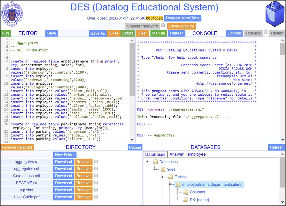
2.3 The Online Interface DESweb
An online system is
available at https://desweb.fdi.ucm.es, where the following
facade is presented:
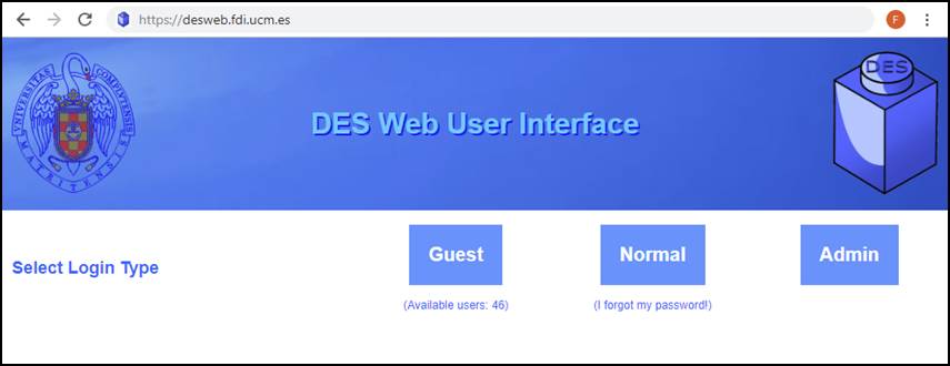
If you do
not have an account, you can login as a guest user (by clicking the first
button Guest) This will open the following interface:
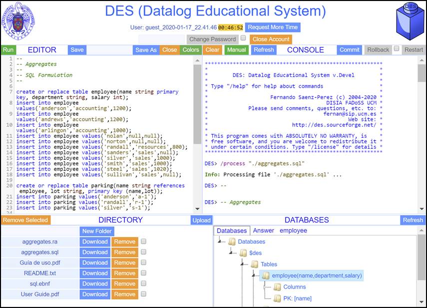
A user
manual (User Guide.pdf) for this interface can be found in the panel DIRECTORY.
3. Getting Started
Whichever
method you use to start DES (a script, batch file, or shortcut, as described in
Section 2.2), you get the following:
|
********************************************************* |
Last line (DES>) is the DES system prompt, which allows you to
write queries and statements in the languages Datalog, SQL, Relational Algebra (RA),
Tuple Relational Calculus (TRC), and Domain Relational Calculus (DRC). Also, commands,
temporary views and conjunctive queries (see next sections) can be inputs. If
an error leads to an exit from DES and you have started from a Prolog
interpreter, then you can write ”des.” (without the double quotes and with the dot) at the Prolog prompt to
continue.
Though a
query in any of the languages above can be submitted from such a prompt, there
are currently six modes available which enable to use a concrete query
interpreter for Datalog, SQL, RA, TRC, DRC and also Prolog (a special mode is
used for fuzzy Datalog, c.f. Section 4.1.22). The Datalog mode is the default. Modes
can be switched with the commands /datalog, /sql, /ra, /trc , /drc and /prolog. Note that commands always start
with a slash (/). Anyway, if you are in a given mode, you can
submit queries or goals to other interpreter simply by writing the query or goal
after any of the previous commands. Also, if you are in Datalog mode, you can
directly submit SQL, RA, TRC and DRC queries. But a Prolog query can only be
submitted from either the Prolog mode or with the command /prolog.
Data are
stored in an in-memory deductive database, including facts (the extensional
database part) and rules (the intensional database part). All queries and goals,
irrespective of the language, refer to this database. When an external database
is opened (see Section 5.1), their tables and views are
available and can be queried from Datalog, Prolog, RA, TRC, DRC and SQL. The
term relation is interchangeably used
with predicate, as are also the terms
goal and query.
In contrast
with interpreters of other systems, the default input mode is single-line,
which means that the input will be processed after hitting the Intro key, which allows to omit the
terminating character. Nonetheless, this mode can be switched to multi-line as
described in Section 5.7 with the command /multiline on. However, even in this mode, commands remain
as single-line inputs.
Terminal
sessions in this manual correspond to actual sessions in a given DES version
(not always the last one). Listings have been captured with compact listings
enabled (with the command /multiline on).
3.1 Datalog Mode
In this
mode, a query is sent to the Datalog processor. If it does not follow Datalog
syntax, then it is sent, first, to the SQL processor (see Section 4.2) , second, to the RA processor (see
Section 4.3), third, to the TRC processor (see
Section 4.4), and fourth, to the DRC processor
(see Section 4.4) should such query is written in
any of these other query languages (See caveats in Section 3.7).
Commands
(see Section 5.17) start with a slash (/) and are sent to the command
processor. Commands can end with an optional dot. While in single-line mode,
Datalog inputs can also end with an optional dot, the dot is required in multi-line
mode. Datalog mode is the default mode and can be anyway enabled via the
command /datalog.
The typical
way of using the system is to write Datalog program files (with default
extension .dl) and consulting them before submitting
queries. Another alternative is to interactively assert program rules in the system
prompt. Following the first alternative, you write the program in a text file,
and then change to the path where the file is located by using the command /cd Path, where Path is the new directory (relative or
absolute). Next, the command /consult FileName is used to consult the file FileName. Or, instead of changing the
current directory, you can write the absolute or relative path to the file in
the consult command. When writing a path, you can use interchangeably the
backslash and the slash to delimit folders in Windows.
Provided that
there are a number or example files in the directory examples at the distribution directory, and assuming
that the current path is the distribution directory (as by default), one can
use the following commands to consult the example file relop.dl:[2]
DES> /cd examples
DES> /consult relop.dl
Info: 18 rules consulted.
(where the default extension .dl can be omitted). Note that Datalog rules in
files must end with a dot, in contrast to command prompt inputs, where the dot
is optional in single-line input. Rules in a consulted file may span on
multiple lines because a multi-line mode is enforced for such files.
Be warned that the command /consult erases the current database. If you want to
keep already loaded facts and rules, use the command /reconsult instead.
Then, one can examine the contents of the database (see Section 6.1 for an explanation of the consulted
program) via the command:
DES> /listing
a(a1).
a(a2).
a(a3).
b(a1).
b(b1).
b(b2).
c(a1,a1).
c(a1,b2).
c(a2,b2).
cartesian(X,Y) :-
a(X),
b(Y).
difference(X) :-
a(X),
not b(X).
full_join(X,Y) :-
fj(a(X),b(Y),X = Y).
inner_join(X) :-
a(X),
b(X).
left_join(X,Y) :-
lj(a(X),b(Y),X = Y).
projection(X) :-
c(X,Y).
right_join(X,Y) :-
rj(a(X),b(Y),X = Y).
selection(X)
:-
a(X),
X = a2.
union(X) :-
a(X)
;
b(X).
Info: 18 rules listed.
Submitting
a query is pretty easy:
DES> a(X)
{
a(a1),
a(a2),
a(a3)
}
Info: 3 tuples computed.
You can
interactively add new rules with the command /assert, as in:
DES> /assert a(a4)
DES> a(X)
{
a(a1),
a(a2),
a(a3),
a(a4)
}
Info: 4 tuples computed.
Saving the
current database, which may include such interactively added (or , if it is the
case, deleted) tuples, is allowed with the command /save_ddb Filename, which saves in a plain file the
Datalog rules located in the default in-memory database. Later, they can be
restored with /restore_ddb Filename (this command is only an alias for /consult.) In the following session, the
current database is stored, abolished (cleared), and finally restored. All the
data, including the ones interactively added are eventually recovered:
DES> /save_ddb db.dl
DES> /abolish
DES> /restore_ddb db.dl
Info: 19 rules consulted.
DES>
a(X)
{
a(a1),
a(a2),
a(a3),
a(a4)
}
Info: 4 tuples computed.
In addition
to be able of saving the in-memory database, Section 5.2 explains how to make single
predicates persistent in external SQL databases.
Another
useful command is /list_et, which lists, in particular, the answers
already computed. Following the last series of queries and commands above, we
submit:
Answers:
{
a(a1),
a(a2),
a(a3),
a(a4)
}
Info: 4 tuples in the answer table.
Calls:
{
a(A)
}
Info: 1 tuple in the call table.
Here, we
can see that the computed meaning of the queried relation is stored in an extension
(answer) table, as well as the last call (cf. sections 5.22.1 and 5.22.2). The extension table keeps
computed results unless either the database is changed (e.g., via /assert, /retract or /abolish commands), or a Datalog temporary
view (see Section 4.1.6) is executed, or an SQL, RA, TRC or
DRC query is executed, or the command /clear_et is submitted.
3.2 SQL Mode
In this mode,
queries are sent to the SQL processor, whereas commands (cf. Section 5.17) are sent to the command processor.
SQL queries can end with an optional semicolon in single-line mode. Multi-line
mode requires the ending semicolon. SQL mode is enabled via the command /sql. Datalog, RA, TRC and DRC queries
cannot be handled by this mode. Recall, however, that the Datalog mode is able
to reckon SQL inputs and handle them without the need for turning on the SQL
mode. The SQL mode is provided for a single language input (cf. Section 3.7) and to display language-specific
syntax errors.
If we want
to develop an analogous SQL example session to the Datalog example in the last
section, we can submit the first inputs (also available in the file examples/relop.sql) listed below (the example is augmented to
provide a first glance of SQL). Now, answer relations to SQL queries are
denoted by the relation name answer. Also note that lines starting by -- are simply remarks as usual in SQL
systems (though you can still use %). If you wish to automatically reproduce the
following interactive session of inputs, you can type /process examples/relop.sql (notice that you must omit examples/ if you are in this directory already):
Info: Processing file
'relop.sql' ...
DES> -- Switch to SQL
interpreter
DES> /sql
DES> -- Creating tables
DES> create or replace table a(a string);
DES> create or replace table b(b string);
DES> create or replace table c(a string,b string);
DES> -- Listing the
database schema
DES> /dbschema
Info: Table(s):
* a(a:string)
* b(b:string)
* c(a:string,b:string)
Info: No views.
Info: No integrity constraints.
DES> -- Inserting values
into tables
DES> insert into a values ('a1');
Info: 1 tuple inserted.
DES> insert into a values ('a2');
Info: 1 tuple inserted.
DES> insert into a values ('a3');
Info: 1 tuple inserted.
DES> insert into b values ('b1');
Info: 1 tuple inserted.
DES> insert into b values ('b2');
Info: 1 tuple inserted.
DES> insert into b values ('a1');
Info: 1 tuple inserted.
DES> insert into c values ('a1','b2');
Info: 1 tuple inserted.
DES> insert into c values ('a1','a1');
Info: 1 tuple inserted.
DES> insert into c values ('a2','b2');
Info: 1 tuple inserted.
DES> -- Testing the just
inserted values
DES> select * from a;
answer(a.a) ->
{
answer(a1),
answer(a2),
answer(a3)
}
Info: 3 tuples computed.
DES> select * from b;
answer(b.b) ->
{
answer(a1),
answer(b1),
answer(b2)
}
Info: 3 tuples computed.
DES> select * from c;
answer(c.a, c.b) ->
{
answer(a1,a1),
answer(a1,b2),
answer(a2,b2)
}
Info: 3 tuples computed.
DES> -- Projection
DES> select a from c;
answer(c.a) ->
{
answer(a1),
answer(a2)
}
Info: 2 tuples computed.
DES> -- Selection
DES> select a from a where a='a2';
answer(a.a) ->
{
answer(a2)
}
Info: 1 tuple computed.
DES> -- Cartesian product
DES> select * from a,b;
answer(a.a, b.b) ->
{
answer(a1,a1),
answer(a1,b1),
answer(a1,b2),
answer(a2,a1),
answer(a2,b1),
answer(a2,b2),
answer(a3,a1),
answer(a3,b1),
answer(a3,b2)
}
Info: 9 tuples computed.
DES> -- Inner Join
DES> select a from a inner join b on a.a=b.b;
answer(a) ->
{
answer(a1)
}
Info: 1 tuple computed.
DES> -- Left Join
DES> select * from a left join b on a.a=b.b;
answer(a.a, b.b) ->
{
answer(a1,a1),
answer(a2,null),
answer(a3,null)
}
Info: 3 tuples computed.
DES> -- Right Join
DES> select * from a right join b on a.a=b.b;
answer(a.a, b.b) ->
{
answer(a1,a1),
answer(null,b1),
answer(null,b2)
}
Info: 3 tuples computed.
DES> -- Full Join
DES> select * from a full join b on a.a=b.b;
answer(a.a, b.b) ->
{
answer(a1,a1),
answer(a1,null),
answer(a2,null),
answer(a3,null),
answer(null,a1),
answer(null,b1),
answer(null,b2)
}
Info: 7 tuples computed.
DES> -- Union
DES> select * from a union select * from b;
answer(a.a) ->
{
answer(a1),
answer(a2),
answer(a3),
answer(b1),
answer(b2)
}
Info: 5 tuples computed.
DES> -- Difference
DES> select * from a except select * from b;
answer(a.a) ->
{
answer(a2),
answer(a3)
}
Info: 2 tuples computed.
Info: Batch file processed.
Duplicates
are disabled by default, i.e., answers are set-oriented. But they can be
enabled as well, which is useful in Datalog, SQL and RA queries (see Section 4.1.9). For instance:
DES> /duplicates on
Info: Duplicates are on.
DES> select a from c;
answer(c.a:string) ->
{
projection(a1),
projection(a1),
projection(a2)
}
Info: 3 tuples computed.
You can see
the equivalent Datalog rules for a given query by enabling compilation listings
as in:
DES> /show_compilations on
DES> select * from a union all select * from b;
Info: SQL statement compiled to:
answer(A) :-
a(A).
answer(A) :-
b(A).
answer(a.a:string) ->
{
answer(a1),
answer(a2),
answer(a3),
answer(b1),
answer(b2)
}
Info: 5 tuples computed.
3.3 Relational Algebra Mode
In this
mode, queries are sent to the Relational Algebra (RA) processor, whereas
commands (cf. Section 5.17) are sent to the command processor.
RA queries can end with an optional semicolon in single-line mode. Multi-line
mode requires the ending semicolon. RA mode is enabled via the command /ra. Datalog, SQL, TRC and DRC queries
cannot be handled by this mode. Recall, however, that the Datalog mode is able
to reckon SQL, RA, TRC and DRC inputs and handle them without the need for
turning on the RA mode. The relational algebra mode is provided for a single
language input (cf. Section 3.7) and to display language-specific
syntax errors.
If we want
to develop an analogous RA example session to the former examples, we can
submit the first inputs (also available in the file examples/relop.ra) listed below. Now, answer relations to RA
queries are denoted by the relation name answer. As before, lines starting by either % or -- are simply remarks. If you wish to automatically reproduce the
following interactive session of inputs, you can type /process examples/relop.ra (notice that you must omit examples/ if the current directory is this one already):
DES> % Creating tables
%
Table creation and tuple insertion are omitted here because they are the same
as in the SQL session in previous Section 3.2.
DES-RA> % Testing the just
inserted values
DES-RA> select true (a);
answer(a.a:string) ->
{
answer(a1),
answer(a2),
answer(a3)
}
Info: 3 tuples computed.
DES-RA> select true (b);
answer(b.b:string) ->
{
answer(a1),
answer(b1),
answer(b2)
}
Info: 3 tuples computed.
DES-RA> select true (c);
answer(c.a:string,c.b:string) ->
{
answer(a1,a1),
answer(a1,b2),
answer(a2,b2)
}
Info: 3 tuples computed.
DES-RA> % Projection
DES-RA> project a (c);
answer(c.a:string) ->
{
answer(a1),
answer(a2)
}
Info: 2 tuples computed.
DES-RA> % Selection
DES-RA> select a='a2'
(a);
answer(a.a:string) ->
{
answer(a2)
}
Info: 1 tuple computed.
DES-RA> % Cartesian product
DES-RA> a product b;
answer(a.a:string,b.b:string) ->
{
answer(a1,a1),
answer(a1,b1),
answer(a1,b2),
answer(a2,a1),
answer(a2,b1),
answer(a2,b2),
answer(a3,a1),
answer(a3,b1),
answer(a3,b2)
}
Info: 9 tuples computed.
DES-RA> % Union
DES-RA> a union b;
answer(a.a:string) ->
{
answer(a1),
answer(a2),
answer(a3),
answer(b1),
answer(b2)
}
Info: 5 tuples computed.
DES-RA> % Difference
DES-RA> a difference b;
answer(a.a:string) ->
{
answer(a2),
answer(a3)
}
Info: 2 tuples computed.
DES-RA> % Intersection
DES-RA> a intersect b;
answer(a.a:string) ->
{
answer(a1)
}
Info: 1 tuple computed.
DES-RA> % Theta Join
DES-RA> select a.a=b.b (a product b);
answer(a.a:string,b.b:string) ->
{
answer(a1,a1)
}
Info: 1 tuple computed.
DES-RA> a zjoin a.a=b.b b;
answer(a.a:string,b.b:string) ->
{
answer(a1,a1)
}
Info: 1 tuple computed.
DES-RA> % Natural Inner Join
DES-RA> a njoin c;
answer(a.a:string,c.b:string) ->
{
answer(a1,a1),
answer(a1,b2),
answer(a2,b2)
}
Info: 3 tuples computed.
DES-RA> % Left Outer Join
DES-RA> a ljoin a.a=b.b b;
answer(a.a:string,b.b:string) ->
{
answer(a1,a1),
answer(a2,null),
answer(a3,null)
}
Info: 3 tuples computed.
DES-RA> % Right Outer Join
DES-RA> a rjoin a.a=b.b b;
answer(a.a:string,b.b:string) ->
{
answer(a1,a1),
answer(null,b1),
answer(null,b2)
}
Info: 3 tuples computed.
DES-RA> % Full Outer Join
DES-RA> a fjoin a.a=b.b b;
answer(a.a:string,b.b:string) ->
{
answer(a1,a1),
answer(a2,null),
answer(a3,null),
answer(null,b1),
answer(null,b2)
}
Info: 5 tuples computed.
DES-RA> % Grouping
DES-RA> group_by a a,count(*) true (c);
answer(c.a:string,$a3:int) ->
{
answer(a1,2),
answer(a2,1)
}
Info: 2 tuples computed.
DES-RA> % Renaming
DES-RA> select a1.a<a2.a ((rename a1(a) (a)) product (rename a2(a) (a)));
answer(a1.a:string,a2.a:string) ->
{
answer(a1,a2),
answer(a1,a3),
answer(a2,a3)
}
Info: 3 tuples computed.
DES-RA> % Duplicate elimination
DES-RA> /duplicates off
Info: Duplicates are already disabled.
DES-RA> project a (c);
answer(c.a:string) ->
{
answer(a1),
answer(a2)
}
Info: 2 tuples computed.
DES-RA> /duplicates on
DES-RA> project a (c);
answer(c.a:string) ->
{
answer(a1),
answer(a1),
answer(a2)
}
Info: 3 tuples computed.
DES-RA> distinct (project a (c));
answer(c.a:string) ->
{
answer(a1),
answer(a1),
answer(a2)
}
Info: 3 tuples computed.
As well,
you can see both the equivalent Datalog rules and SQL statement for a given RA
query by enabling compilation listings and SQL display as in:
DES> /show_compilations on
DES> /show_sql on
DES> a union b
Info: Equivalent SQL query:
(
SELECT ALL *
FROM
a
)
UNION ALL
(
SELECT ALL *
FROM
b
);
Info: RA expression compiled to:
answer(A) :-
a(A).
answer(A) :-
b(A).
answer(a.a:string) ->
{
answer(a1),
answer(a2),
answer(a3),
answer(b1),
answer(b2)
}
Info: 5 tuples computed.
3.4 Tuple Relational Calculus Mode
In this mode,
queries are sent to the Tuple Relational Calculus (TRC) processor, whereas
commands (cf. Section 5.17) are sent to the command processor.
TRC queries can end with an optional semicolon in single-line mode. Multi-line
mode requires the ending semicolon. TRC mode is enabled via the command /trc. Datalog, SQL, RA and DRC queries
cannot be handled by this mode. Recall, however, that the Datalog mode is able
to reckon SQL, RA, TRC and DRC inputs and handle them without the need for
turning on the TRC mode. The tuple relational calculus mode is provided for a
single language input (cf. Section 3.7) and to display language-specific
syntax errors.
If we want
to develop an analogous TRC example session to the former examples, we can
submit the first inputs (also available in the file examples/relop.trc) listed below. Now, answer relations to TRC
queries are denoted by the relation name answer. As before, lines starting by either % or -- are simply remarks. If you wish to automatically reproduce the
following interactive session of inputs, you can type /process examples/relop.trc (notice that you must omit examples/ if you are in this directory already):
DES> % Creating tables
%
Table creation and tuple insertion are omitted here because they are the same
as in the SQL session in previous Section 3.2.
DES-TRC> % Testing the just
inserted values
DES-TRC>
{A|a(A)};
Info: TRC statement compiled to:
answer(A) :-
a(A).
answer(a:string) ->
{
answer(a1),
answer(a2),
answer(a3)
}
Info: 3 tuples computed.
DES-TRC>
{B|b(B)};
Info: TRC statement compiled to:
answer(B) :-
b(B).
answer(b:string) ->
{
answer(a1),
answer(b1),
answer(b2)
}
Info: 3 tuples computed.
DES-TRC>
{C|c(C)};
Info: TRC statement compiled to:
answer(A,B) :-
c(A,B).
answer(a:string,b:string) ->
{
answer(a1,a1),
answer(a1,b2),
answer(a2,b2)
}
Info: 3 tuples computed.
DES-TRC> % Projection
DES-TRC>
{C.a|c(C)};
Info: TRC statement compiled to:
answer(A) :-
c(A,_B).
answer(a:string) ->
{
answer(a1),
answer(a2)
}
Info: 2 tuples computed.
DES-TRC> % Selection
DES-TRC>
{A|a(A) and A.a='a2'};
Info: TRC statement compiled to:
answer(A) :-
a(A),
A=a2.
answer(a:string) ->
{
answer(a2)
}
Info: 1 tuple computed.
DES-TRC> % Cartesian product
DES-TRC> {A,B|a(A) and b(B)};
Info: TRC statement compiled to:
answer(A,B) :-
a(A),
b(B).
answer(a:string,b:string) ->
{
answer(a1,a1),
answer(a1,b1),
answer(a1,b2),
answer(a2,a1),
answer(a2,b1),
answer(a2,b2),
answer(a3,a1),
answer(a3,b1),
answer(a3,b2)
}
Info: 9 tuples computed.
DES-TRC> % Union
DES-TRC>
{X|a(X) or b(X)};
Info: TRC statement compiled to:
answer(A) :-
a(A)
;
b(A).
answer(a:string) ->
{
answer(a1),
answer(a2),
answer(a3),
answer(b1),
answer(b2)
}
Info: 5 tuples computed.
DES-TRC> % Difference
DES-TRC>
{X|a(X) and not b(X)};
Info: TRC statement compiled to:
answer(A) :-
a(A),
not b(A).
answer(a:string) ->
{
answer(a2),
answer(a3)
}
Info: 2 tuples computed.
DES-TRC> % Intersection
DES-TRC>
{X|a(X) and b(X)};
Info: TRC statement compiled to:
answer(A) :-
a(A),
b(A).
answer(a:string) ->
{
answer(a1)
}
Info: 1 tuple computed.
DES-TRC> % Theta Join
DES-TRC> {A,B|a(A) and b(B) and A.a=B.b};
Info: TRC statement compiled to:
answer(A,B) :-
a(A),
b(B),
A=B.
answer(a:string,b:string) ->
{
answer(a1,a1)
}
Info: 1 tuple computed.
DES-TRC> % Natural Inner Join
DES-TRC> {A.a,C.b|a(A) and c(C) and A.a=C.a};
Info: TRC statement compiled to:
answer(A,B) :-
a(A),
c(_C_a,B),
A=_C_a.
answer(a:string,b:string) ->
{
answer(a1,a1),
answer(a1,b2),
answer(a2,b2)
}
Info: 3 tuples computed.
3.5 Domain Relational Calculus Mode
In this
mode, queries are sent to the Domain Relational Calculus (DRC) processor,
whereas commands (cf. Section 5.17) are sent to the command processor.
DRC queries can end with an optional semicolon in single-line mode. Multi-line
mode requires the ending semicolon. DRC mode is enabled via the command /drc. Datalog, SQL, RA and TRC queries
cannot be handled by this mode. Recall, however, that the Datalog mode is able
to reckon SQL, RA, TRC and DRC inputs and handle them without the need for
turning on the DRC mode. The tuple relational calculus mode is provided for a
single language input (cf. Section 3.7) and to display language-specific
syntax errors.
If we want
to develop an analogous DRC example session to the former examples, we can
submit the first inputs (also available in the file examples/relop.drc) listed below. Now, answer relations to TRC
queries are denoted by the relation name answer. As before, lines starting by either % or -- are simply remarks. If you wish to automatically reproduce the
following interactive session of inputs, you can type /process examples/relop.drc (notice that you must omit examples/ if you are in this directory already):
DES> % Creating tables
%
Table creation and tuple insertion are omitted here because they are the same
as in the SQL session in previous Section 3.2.
DES-DRC> % Testing the just
inserted values
DES-DRC>
{A|a(A)};
Info: DRC statement compiled to:
answer(A) :-
a(A).
answer(a:string) ->
{
answer(a1),
answer(a2),
answer(a3)
}
Info: 3 tuples computed.
DES-DRC>
{B|b(B)};
Info: DRC statement compiled to:
answer(B) :-
b(B).
answer(b:string) ->
{
answer(a1),
answer(b1),
answer(b2)
}
Info: 3 tuples computed.
DES-DRC> {A,B|c(A,B)};
Info: DRC statement compiled to:
answer(A,B) :-
c(A,B).
answer(a:string,b:string) ->
{
answer(a1,a1),
answer(a1,b2),
answer(a2,b2)
}
Info: 3 tuples computed.
DES-DRC> % Projection
DES-DRC>
{A|c(A,_)};
Info: DRC statement compiled to:
answer(A) :-
c(A,_).
answer(a:string) ->
{
answer(a1),
answer(a2)
}
Info: 2 tuples computed.
DES-DRC> % Selection
DES-DRC>
{A|a(A) and A>='a2'};
Info: DRC statement compiled to:
answer(A) :-
a(A),
A>=a2.
answer(a:string) ->
{
answer(a2),
answer(a3)
}
Info: 2 tuples computed.
DES-DRC> % Cartesian product
DES-DRC> {A,B|a(A) and b(B)};
Info: DRC statement compiled to:
answer(A,B) :-
a(A),
b(B).
answer(a:string,b:string) ->
{
answer(a1,a1),
answer(a1,b1),
answer(a1,b2),
answer(a2,a1),
answer(a2,b1),
answer(a2,b2),
answer(a3,a1),
answer(a3,b1),
answer(a3,b2)
}
Info: 9 tuples computed.
DES-DRC> % Union
DES-DRC>
{A|a(A) or b(A)};
Info: DRC statement compiled to:
answer(A) :-
a(A)
;
b(A).
answer(a:string) ->
{
answer(a1),
answer(a2),
answer(a3),
answer(b1),
answer(b2)
}
Info: 5 tuples computed.
DES-DRC> % Difference
DES-DRC>
{A|a(A) and not b(A)};
Info: DRC statement compiled to:
answer(A) :-
a(A),
not b(A).
answer(a:string) ->
{
answer(a2),
answer(a3)
}
Info: 2 tuples computed.
DES-DRC> % Intersection
DES-DRC> {A|a(A)
and b(A)};
Info: DRC statement compiled to:
answer(A) :-
a(A),
b(A).
answer(a:string) ->
{
answer(a1)
}
Info: 1 tuple computed.
DES-DRC> % Theta Join
DES-DRC> {A,B|a(A) and b(B) and A>=B};
Info: DRC statement compiled to:
answer(A,B) :-
a(A),
b(B),
A>=B.
answer(a:string,b:string) ->
{
answer(a1,a1),
answer(a2,a1),
answer(a3,a1)
}
Info: 3 tuples computed.
DES-DRC> % Natural Inner Join
DES-DRC> {A,B|a(A) and c(A,B)};
Info: DRC statement compiled to:
answer(A,B) :-
a(A),
c(A,B).
answer(a:string,b:string) ->
{
answer(a1,a1),
answer(a1,b2),
answer(a2,b2)
}
Info: 3 tuples computed.
3.6 Prolog Mode
This mode
is enabled via the command /prolog and goals are sent to the Prolog processor. This
is the only language mode in which Prolog inputs can be processed. Assuming
that the file relop.dl has been already consulted, let’s consider
the following example:
DES-Prolog>
projection(X)
projection(a1)
?
(type ; for more solutions, <Intro> to continue) ;
projection(a1)
?
(type ; for more solutions, <Intro> to continue) ;
projection(a2)
?
(type ; for more solutions, <Intro> to continue) ;
no
DES-Prolog> /datalog projection(X)
{
projection(a1),
projection(a2)
}
Info: 2 tuples computed.
The
execution of this goal allows to noting the basic differences between Prolog
and Datalog engines. First, the former searches for solutions, one-by-one, that
satisfy the goal projection(X). The latter gives the whole meaning[3] of the user-defined relation projection with the query projection(X) at a time. And, second, note the default
set-oriented behaviour of the Datalog engine, which discards duplicates in the
answer.
3.7 Caveats
Since the Datalog mode prompt accepts Datalog, SQL, RA,
TRC and DRC queries, a given query can be interpreted in more than one language.
Let's consider the following system session, in which a table is created and an
RA query is submitted:
DES> create table t(a int)
DES> insert into t values(1)
DES> distinct (t)
Info: Processing:
answer :-
distinct(t).
Warning: Undefined predicate(s): [t/0]
{
}
Info: 0 tuples computed.
Here, we get a missing answer as we’d expect the tuple
t(1) in
the result set. However, this query has been processed as a Datalog one, where distinct (t) computes the different tuples for the relation t/0 (which is not defined in this
system session). To overcome such situations, simply precede the query by the
language selection command, as follows:
DES> /ra distinct (t)
answer(t.a:int) ->
{
answer(1)
}
Info: 1 tuple computed.
Alternatively, switch to the other query processor:
DES> /ra
DES-RA> distinct (t)
Another example is the division operator:
DES> create table t(a int, b int)
DES> create table s(a int)
DES> t division s
Error: Incompatible schemas in division operation: t division s
DES> /ra t division s
answer(t.b:int) ->
{
}
Info: 0 tuples computed.
As the query t division s is firstly interpreted as a
Datalog query, both t and s are
assumed to be predicates of arity 0, which obviously are not compatible for the
operation. Prepending the command /ra forces the system to interpret the input as an RA query, providing the
expected result.
3.8 Getting Help
You can get
useful information with the following commands:
·
/help. Shows the list of available commands, which
are explained in Section 5.17.
·
/help Keyword. To request help on a given keyword
(command or built-in).
·
/builtins. Shows the list of built-ins, which are
explained in Section 4.7.
If the
system can find appropriate names for those which are not valid, it
automatically informs the user. In particular, if a given predicate does not
exist but some similar names are found (modulo misspelling), they are hinted to
the user. Another hints include alternative column, table and view names are
for SQL DML and DDL queries and Datalog queries. This is somewhat related to
SWI-Prolog's DWIM (Do What I Mean).
Also, visit
the URL for last information:
http://des.sourceforge.net/
Finally,
you can contact the author via the e-mail address:
fernan@sip.ucm.es
4. Query Languages
DES has
evolved from a quite simple Datalog interpreter to its current state, a system
relying on a deductive database engine which can be queried with either Datalog,
SQL, RA, TRC and DRC languages. In addition, a Prolog interface is also
provided in order to highlight the differences between Datalog and Prolog
systems. Since DES is intended to students, it has no full-blown features of either
state-of-the-art Prolog, or Datalog or SQL-based systems. However, it has many
features that make it appealing as an educational tool, along with the novel
implementations of declarative debugging (sections 5.10 and 5.11) and the test case generator
(Section 0). In this section, we describe its four
query languages: Datalog, SQL, RA, and Prolog.
The
database is shared by all the query languages, so that queries or goals can
refer to any object defined using any language. However, there are some
dependent issues that must be taken into account. For instance, once a Datalog
fact is loaded into the database, the relation it defines can be queried in
Datalog. But, if one wants to access this relation from either SQL, or RA, or
TRC or DRC, two alternatives are provided: 1) Define the same relation in SQL
via a create
table statement
(Section 4.2.4.1), and 2) Declare types for the
table (Section 4.1.18.1). This particular issue comes from
the fact that Datalog relations have unnamed attributes, and a positional
reference based on variables (instead of indexes) is used for accessing those relations.
In turn, SQL, RA, TRC and DRC use a notational syntax, giving names to relation
arguments. To illustrate the first alternative, let’s consider the following
session:
DES> /assert t(1)
DES> t(X)
{
t(1)
}
Info: 1 tuple computed.
DES> select * from t
Error: Unknown table or view "t"
DES> create table
t(a int);
DES> select * from t;
answer(t.a:int) ->
{
answer(1)
}
Info: 1 tuple computed.
The error
above reflects that t is not a known object for SQL
statements in the database schema.
Following the
second alternative to access a Datalog relation from SQL:
DES> /assert t(1)
DES> :-type(t,[a:int])
DES> select * from t
answer(t.a:int) ->
{
answer(1)
}
Info: 1 tuple computed.
4.1 Datalog
Since
Datalog stems from Prolog, we have adopted almost all the Prolog syntax
conventions for writing Datalog programs (the reader is assumed to have basic
knowledge about Prolog). Syntax follows Prolog ISO standard [ISO00]
(considering Datalog syntax as a subset of Prolog). We allow (recursive)
Datalog programs with stratified negation [Ullm95], i.e., normal logic programs
without function symbols. Stratification is imposed to ensure a clear semantics
when negation is involved, and function symbols are not allowed in order to
guarantee termination of queries, a natural requirement with respect to a (relational)
database user who is not able to deal with compound data.
Commands
are somewhat different for Prolog programmers as they are accustomed to (see
Section 5.17). Also, exceptions are noted when
necessary.
4.1.1 Syntax
Definitions
for Datalog mainly come from the field of Logic Programming, following [Lloyd87],
referring the reader to this book for a more general presentation of Logic
Programming. Next, some definitions for understanding the syntax of programs,
queries and views are introduced.
·
Numbers. Integers and float numbers are allowed. A
number is a float whenever the number contains a dot (.) between two digits. The range depends on the Prolog platform being
used. Negative numbers are identified by a preceding minus (-), as usual.
Scientific notation is supported, as usually,
in E-notation as: mEn, where m is a number (maybe including a fractional part), and n is an integer, which may start with + or – (but it is not required). The base (10) can be represented with either E or e.
If the fractional dot is included in a number,
there must be (at least) a digit to its left and another to its right.
Examples of numbers are 1, 1.1, -1.0, 1.2E34, 1.2E+34, and 0.2e-34.
Note that -1., +1, .1, 1.E23, and 1E2.3 are not valid numbers. A plus sign is not part
of a positive number; however, both a plus and a minus sign can be used as a
prefix unary operator in arithmetical expressions (cf. Section 4.7.4.1) and also following the symbol E in scientific notation, as already seen.
·
Constants. A constant can be:
o
A
number (either integer or float).
o
Any
sequence of alphanumeric characters (including the underscore _), starting with a lowercase letter.
o
Any
sequence of characters delimited by single quotes. If the sequence contains a
single quote, it can be either escaped or to be included as part of the
constant.
Examples of alphanumeric constants are foo, foo_foo, 'foo foo',
'2*3', 'X', 'foo''s', and 'foo\'s'. The last two represent the same constant (foo's).
·
Variables. Variables are written with
alphanumeric characters, and alternatively start with either an uppercase or
with an underscore (_). Anonymous variables are also
allowed, which are denoted with a single underscore. Each occurrence of an
anonymous variable is considered different from any other variable (either anonymous
or not). For instance, in the rule a :- b(_), c(_), goals do not share variables. Any variable starting with an underscore
(either anonymous or not) is removed from the answer to a query (cf. Section 4.1.7). Also, they are not taken into
account for singleton variable warnings (cf. Section 5.5.5).
Examples of variables are: X, _X, _var, and
_.
· Unknowns. Unknowns are
represented as null values and are written alternatively as both null and '$NULL'(ID), where ID is a
unique global identifier. The first form is used for normal users, whilst the
second one is intended for development uses (cf. /development command
in Section ).
·
Operators.
o
Infix,
as addition (e.g., 1+2).
o
Prefix,
as bitwise negation (e.g., \1).
Available operators (comparisons, arithmetic,
string, and date/time) can be consulted in Section 4.7.
· Terms. Terms
can be:
o Non-compound. Variables or constants.
o
Compound. As in Prolog, they have
the form t(t1, ..., tn),
where t is a function symbol (functor), and ti (1 ≤
i
≤ n) are terms. Compound terms are very restricted
in DES and can only be of the following forms:
§
'$NULL'(ID) for internally representing nulls.
§ Date/time data values, with the form
explained in Section 4.1.18.1.
§
Predicate
patterns of the form Name/Arity for fuzzy proximity equations (see Section 4.1.22.1).
Examples of
terms are: r(p), and p(X,Y), and X > Y.
·
Expressions. An expression is constructed with constants, operators, and functions.
An expression occurring in any comparison operator is evaluated before applying
the comparison. There is one exception: the operator \== (intended for syntactic disequality) which do not evaluate their
arguments. Expressions can be of different data types (integer, string, ...).
Examples of expressions are:
1/2, 10*rand, length('Hello'), year(current_date) and 'Hello, ' || 'world'
Refer to Section 4.7 for available built-in functions.
·
Atoms. An atom has the form a(t1, ..., tn), where a is a predicate (relation) symbol,
and ti (1 ≤ i ≤ n) are terms. If i is 0, then the atom is simply written as a.
Positive, ground atoms are used to build the Herbrand universe.
There are several built-in predicates: is (for evaluating arithmetical expressions), arithmetic functions, (infix
and prefix) operators and constants, and comparison operators. Comparison
operators are infix, as “less-than”. For example, 1 < 2 is a positive atom built from an infix built-in comparison operator
(see Section 4.7.1).
Examples of atoms are: p, r(a,X), 1 < 2, and X is 1+2.
Note that p(1+2) and p(t(a)) are not valid
atoms.
·
Restricted
atoms. A
restricted atom has the form -A, where A is an atom built with no built-in.
·
Conditions. A condition is a Boolean expression
containing conjunctions (,/2), disjunctions (;/2), built-in comparison operators, constants and variables.
Examples
of conditions are:
X>1, X=Y, (X>Y,Y>Z), (X=<Y;Z<0), and log(X)<sin(pi/2)
Note that the last example is valid because
the arguments of the disequality are evaluable arithmetic expressions, and it
can be solved whenever the rule where it occurs is safe (cf. Section 5.3).
·
Relation
functions. A
function has the form f(a1, …, an), where f is a function name, ai are its arguments, and maps to a relation.
Only built-in functions are allowed. The current provision of built-in relation
functions includes, among others:
o lj(a1,a2,a3). Compute the left outer join
of the relations a1 (left relation) and a2 (right relation), committing the condition (Boolean expression) a3 (join condition).
o order_by(a1,a2). Return the meaning of a1 (left relation) and a2 is the list [E1,..,En], where Ei are ordering expressions (non-declarative function).
o distinct(a1,a2). Return the distinct tuples in the meaning of a2 with respect to the tuple of arguments defined in a2 as the list [V1,..,Vn], where Vi are variables.
Note that outer join functions can be nested (see Section 4.1.11).
·
Literals. Literals can be:
o Positive. An atom or restricted
atom.
o Negative. A negated body of the form
not Body, where Body is a body (cf. next section). Negative literals are used to express the
negation (not truly classical negation) of a relation either as a query or as a
part of a rule body.
o Disjunctive. A disjunctive literal
is of the form l;r , where l and r are literals.
o Divided. A divided literal is of the
form l division r, where l and r are literals.
Examples of literals are:
p
-p
r(a,X)
not q(X,b)
not (a;b)
r(a,X);not q(X,b)
1 < 2
t(X,Y) division s(Y)
X is 1+2
A literal can occur in rule bodies, queries, and view bodies.
Syntax of built-ins is explained in their corresponding forthcoming
sections.
4.1.2 Rules
Datalog rules have the form head :-
body, or simply head. In this last case, the rule is known as a fact. Both end with a dot. A
Datalog head is either an atom or restricted atom (an atom preceded by the
minus sign, cf. Section 4.1.19) that uses no
built-in predicate symbol. A Datalog body contains a comma-separated sequence
of literals, which may contain built-in symbols as listed in Section 4.7, as well as
disjunctions (;/2) and divisions (division/2). A rule with a restricted atom as its head is called a restricting
rule.
4.1.3 Programs
DES programs consist of a multiset
of rules. Programs may contain remarks. A single-line remark starts with the
symbol %, and ends at the end of line. Consulted programs can also contain
multi-line remarks, enclosed between /* and */, which can be nested.
4.1.4 Queries
A (positive)
query is the name of a relation with as many arguments as the arity of the
relation (a positive literal). Each one of these arguments can be a variable or
a constant; a compound term is not allowed but as an arithmetic expression.
Built-in relations may require relations, lists of variables or expressions,
and conditions as arguments. A negative query is written as not Query.
Queries are
typed at the DES system prompt and cannot be part of consulted files, but they
can be part of processed files. The answer to a query is the (multi)set of atoms
matching the query which are deduced in the context of the program, from both
the extensional and the intensional databases. A query with variables for all
the arguments of the queried relation gives the whole set of deduced facts
(meaning) defining the relation, as the query a(X) in
the example of Section 3. If a query contains a constant in
an argument position, it means that the query processing will select the facts
from the meaning of the relation such that the argument position matches with
that constant (i.e., analogous to a select relational operation). This is the
case of the query a(a3) in the same example before.
You can also write conjunctive queries on the fly, such as a(X),
b(X) (see Section 4.1.6). Built-in comparison operators (listed in Section 4.7.1) can be safely used in queries whenever their arguments are ground at
evaluation time (equality does not require this for atomic arguments as it performs
unification; cf. Section 4.7.1 for more details about equality). Disjunctive queries are also allowed
too, as a(X); b(X). A query
follows the same syntax as rule bodies.
If only a limited number of tuples in the
answer are required, one can submit a query as top(N,Query), where N is the maximum number of tuples to be returned (See also offset predicate and Section 4.7.13). Also, query answers can be sorted with order_by (See Section 0). Duplicates can be discarded with distinct (See Section 4.1.9).
4.1.5 Temporary Views
A temporary
view allows you to write a query on the fly, and provide a relation name and
its arguments at will. A temporary view is therefore a rule which is added to
the database; its head is considered as a query and executed. Afterwards, the
rule is removed. Temporary views are useful for quickly submitting conjunctive
queries and for testing the impact of adding a rule to a current relation. For
instance, the view:
DES> d(X) :- a(X), not b(X)
computes the set difference between the sets a and b, provided they have been already defined.
Note that
the view is evaluated in the context of the program; so, if you have more rules
already defined with the same name and arity of the rule's head, the evaluation
of the view will return its meaning under the whole set of rules matching the
query. For instance:
DES> a(X) :- b(X)
computes the set union of the sets a and b, provided they have been already defined.
4.1.6 Automatic Temporary Views
Automatic
temporary views, autoviews for short, are temporary views which do not need a
head and allows you to write conjunctive queries on the fly. When you write a
conjunctive query, a new temporary relation, named answer, is built with as many arguments as
relevant variables occur in the conjunctive query. The identifier answer is a reserved word and cannot be
used for defining any other relation. As an example of an autoview, let’s
consider:
DES> a(X),b(Y)
Info: Processing:
answer(X,Y) :-
a(X),
b(Y).
{
answer(a1,a1),
answer(a1,b1),
answer(a1,b2),
answer(a2,a1),
answer(a2,b1),
answer(a2,b2),
answer(a3,a1),
answer(a3,b1),
answer(a3,b2)
}
Info: 9 tuples computed.
which computes the Cartesian product of the relations a and b, provided they have been already defined as:
a(a1).
a(a2).
a(a3).
b(b1).
b(b2).
b(a1).
4.1.7 Underscored Variables
An underscored
variable (a variable starting with the underscore symbol '_') is handled similar to Prolog. It is assumed to be of no interest for
the answer, so that they are discarded from the answer should they occur in the
body of a query, view or autoview (even in its head)[4]. A special case of underscored
variables is the anonymous variable, which is simply written as '_' (without the quotes). Several occurrences of the anonymous variable in
the same rule are understood as different
variables.
For
instance, computing the projection of a relation t with respect to its first argument can be simply done as follows:
DES> /assert t(1,2)
DES> /assert t(2,3)
DES> t(X,_)
Info: Processing:
answer(X) :-
t(X,_).
{
answer(1),
answer(2)
}
Info: 2 tuples computed.
instead of having to resort to a temporary view such as:
DES> p(X):-t(X,Y)
Info: Processing:
p(X) :-
t(X,Y).
{
p(1),
p(2)
}
Info: 2 tuples computed.
Also, let's
consider other situation, as follows:
DES> /duplicates off
DES> t(X,Y)
{
t(1,1),
t(1,2),
t(3,3)
}
Info: 3 tuples computed.
DES> t(X,X)
{
t(1,1),
t(3,3)
}
Info: 2 tuples computed.
DES> t(_X,_X)
Info: Processing:
answer :-
t(_X,_X).
{
answer
}
Info: 1 tuple computed.
Above, when
underscored variables are used in the query, then you get only one answer tuple.
However, if duplicates are enabled, you get two answer tuples, although the
concrete values for the arguments of t are not
visible:
DES> /duplicates on
DES> t(_X,_X)
Info: Processing:
answer :-
t(_X,_X).
{
answer,
answer
}
Info: 2 tuples computed.
By using
anonymous variables in this query, the result becomes different:
DES> t(_,_)
Info: Processing:
answer :-
t(_,_).
{
answer,
answer,
answer
}
Info: 3 tuples computed.
In this
example, the two arguments of t are not constrained to be equal. Therefore,
you get three answers, one for each tuple in the relation.
As a final
example, the next temporary view gets its head argument removed because _X is considered as a non-relevant variable for the outcome:
DES> v(_X):-p(_X)
Info: Processing:
v :-
p(_X).
{
v
}
Info: 1 tuple computed.
4.1.8 Negation
DES ensures that negative information can be gathered from a program
with negated goals, provided that a restricted form of negation is used: Stratified
negation [Ullm95]. This broadly means that negation is not involved in a
recursive computation path, although it can use recursive rules. The following
program[5] illustrates this point:
a :- not b.
b :- c,d.
c :- b.
c.
The query a succeeds with the meaning {a}. Observe also that not a does not succeed, i.e., its meaning
is the empty set.
If you are interested in how programs with negation are solved, you can
find useful the following commands (cf. Section ):
DES> /pdg
Nodes:
[a/0,b/0,c/0,d/0]
Arcs
: [b/0+c/0,b/0+d/0,c/0+b/0,a/0-b/0]
DES> /strata
[(b/0,1),(c/0,1),(d/0,1),(a/0,2)]
The first command shows the predicate dependency graph (see, e.g.,
[ZCF+97]) for the loaded program. First, nodes in the graph are shown in a list
whose elements P are predicates with their arities with the form
predicate/arity. Next, arcs in the graph are shown in a list whose elements are
either P+Q or P-Q, where P and Q are nodes in the graph. An arc P+Q means that
there exists a rule such that P is the predicate for its head, and Q is the
predicate for one of its literals. If the literal is negated, the arc is
negative, which is expressed as P-Q. The graph for this program can be depicted
as in Figure 1.

Figure 1. Predicate Dependency Graph for negation.dl
The second command shows the stratum assigned to each predicate. This
assignment is computed by following an algorithm based on [Ullm95], but
modified for taking advantage of the predicate dependency graph. Strata are
shown as a list of pairs (P,S), where P is a predicate and S is its assigned
stratum. In this example, all of the program predicates are in stratum 1 but a, which is assigned to stratum 2.
This means that if the meaning of a is to be computed, then the
meanings of predicates in lower strata (and only those predicates a depends on) have to be firstly
computed.
Since the algorithm strata does not follow a naïve bottom-up
solving, only the meanings of required predicates are computed. To illustrate
this, consider the query b for the same program. DES computes
the predicate dependency subgraph for b, i.e., all of the predicates which
are reachable from b, and, then, a stratification is computed.
Notice the different information given by the system for solving the queries a and b (here, verbose output is enabled
with the command /verbose on):
DES> a
Info: Parsing query...
Info: DL query successfully parsed.
Info: Solving query a...
Info: Computing by stratum: [b].
Info: Displaying query answer...
Info: Sorting answer...
{
a
}
Info: 1 tuple computed.
DES> b
Info: Parsing query...
Info: DL query successfully parsed.
Info: Solving query b...
Info: Displaying query answer...
Info: Sorting answer...
{
}
Info: 0 tuples computed.
For the goal a, the system informs that b is previously computed
(nevertheless taking advantage of the extension table mechanism), whereas for
the goal b there is no need of resorting to
the stratum-by-stratum solving.
Finally, see also Section 5.3 for limitations in the use of negation.
4.1.9 Duplicates
Duplicates in answers are removed by default. However, it is also
possible to enable them with the command /duplicates on for Datalog, SQL, and RA. This
allows to generate answers as multisets instead of as the typical set-oriented
deductive systems behave. Computing the meaning of a relation containing
duplicates in the extensional database (i.e., its facts) will include all of
them in the answer, as in:
DES> /duplicates on
DES> /assert t(1)
DES> /assert t(1)
DES> t(X)
{
t(1),
t(1)
}
Info: 2 tuples computed.
Rules can also be source of duplicates, as in:
DES> /assert s(X):-t(X)
DES> s(X)
{
s(1),
s(1)
}
Info: 2 tuples computed.
In particular, recursive rules are duplicate sources, as in:
DES> /assert t(X):-t(X)
DES> t(X)
{
t(1),
t(1),
t(1),
t(1)
}
Info: 4 tuples computed.
where two tuples directly come from the two facts for t/1, and the other two from the
single recursive rule. Again, adding the same recursive rule yields:
DES> /assert t(X):-t(X)
DES> t(X)
{
t(1),
t(1),
t(1),
t(1),
t(1),
t(1),
t(1),
t(1),
t(1),
t(1)
}
Info: 10 tuples computed.
where this answer contains the outcome due to two tuples directly from
the two facts, and four tuples for each recursive rule. The first recursive
rule is source of four tuples because of the two facts and the two tuples from
the second recursive rule. Analogously, the second recursive rule is source of
another four tuples: two facts and the two tuples from the first recursive
rule.
The rule of thumb to understand duplicates in recursive rules is to
consider all possible computation paths in the dependency graph, stopping when
a (recursive) node already used in the computation is reached.
It is also possible to discard duplicates for an atom with the
metapredicate distinct/1. For instance, let’s consider the
following with the same example above:
DES> distinct(t(X))
Info: Processing:
answer(X) :-
distinct(t(X)).
{
answer(1)
}
Info: 1 tuple computed.
Such query is equivalent to the following SQL statement, provided that
metadata is available for the relation t:
DES> :-type(t(a:int))
DES> select distinct * from t
answer(t.a) ->
{
answer(1)
}
Info: 1 tuple computed.
As it would be expected, duplicates are only discarded for the call distinct(Atom), but not for other occurrences of Atom during query solving. Thus:
DES> t(X),distinct(t(X))
Info: Processing:
answer(X) :-
t(X),
distinct(t(X)).
{
answer(1),
answer(1),
answer(1),
answer(1),
answer(1),
answer(1),
answer(1),
answer(1),
answer(1),
answer(1)
}
Info: 10 tuples computed.
Compare this to the call:
DES> t(X),t(X)
Info: Processing:
answer(X) :-
t(X),
t(X).
{
answer(1),
...
answer(1)
}
Info: 100 tuples computed.
A subset of arguments in an atom can be selected for discarding
duplicates. To this end, the metapredicate distinct/2 is provided. Its first argument
is the list of variables for which duplicates are not required, i.e., each
concrete assignment of values to all variables in the list must be different.
So, let's consider the following session:
DES> /listing
t(1,1).
t(1,2).
t(2,1).
Info: 3 rules listed.
DES> distinct([X],t(X,Y))
Info: Processing:
answer(X) :-
distinct([X],t(X,Y)).
{
answer(1),
answer(2)
}
Info: 2 tuples computed.
In addition, discarding duplicates can be performed in the context of
aggregates:
DES> count(distinct(t(X)),C)
Info: Processing:
answer(C)
in the program context of the exploded
query:
answer(C) :-
count('$p0'(X),[],C).
'$p0'(A) :-
distinct(t(A)).
{
answer(1)
}
Info: 1 tuple computed.
See also Section 4.1.12 for discarding duplicates in aggregates.
4.1.10 Null Values
The null value is included in each program signature for denoting
unknowns, in a similar way it is an inherent part of current SQL database
systems. Comparing null values in Datalog opens a new scenario: Two null values
are not (known to be) equal, and are (not known to be) distinct. The following
illustrates this expected behaviour:
DES> null=null
{
}
Info: 0 tuples computed.
DES> null\=null
{
}
Info: 0 tuples computed.
However, for the same null value, the equality should succeed, as in the
conjunctive query: X=null,X=X.
A null value is internally represented as '$NULL'(ID), where ID is a
unique identifier (an integer). Development listings (enabled via the command /development on) allow
to inspect these identifiers, such as in:
DES> /development on
DES> p(X,Y):-X=null,Y=null,X=Y
Info: Processing:
p(X,Y) :-
X = '$NULL'(14),
Y = '$NULL'(15),
X = Y.
{
}
Info: 0 tuples computed.
DES> p(X,Y):-X=null,Y=null,X\=Y
Info: Processing:
p(X,Y) :-
X = '$NULL'(16),
Y = '$NULL'(17),
X \= Y.
{
}
Info: 0 tuples computed.
The built-in predicate is_null/1 tests whether its single argument
is a null value:
DES> is_null(null)
{
is_null(null)
}
Info: 1 tuple computed.
DES> X=null,is_null(X)
Info: Processing:
answer(X) :-
X = null,
is_null(X).
{
answer(null)
}
Info: 1 tuple computed.
Its counterpart predicate is also provided: is_not_null/1, which is true if its argument is
not a null value.
Note that from a system implementor viewpoint, nulls can never unify
because they are represented by different ground terms. On the other hand,
disequality is explicitly handled in order to fail when comparing nulls.
Evaluation of a given expression including at least one null value
returns another different concrete null value n. The very same expression in a further computation step receives
the same null value n. For instance, X=null, X+1=X+1 succeeds, whereas neither X=null, X+1=1+X, nor X=null, Y=null, X+1=Y+1 succeeds.
4.1.11 Outer Joins
Three outer join operations are provided (cf. Section 4.7.9), following relational database query
languages (SQL and extended relational algebra): left (lj/3), right (rj/3) and full (fj/3) outer join. For all these
predicates, their first argument is the argument to the left for the algebra
relational outer join operator, the second argument is the argument to the
right, and the third argument is the condition for the join operation. For
example, lj(L,R,C) represents L ![]()
![]() C R.
C R.
Having loaded the example program relop.dl, we can submit the following
queries:
DES> /c relop
DES> /listing a
a(a1).
a(a2).
a(a3).
DES> /listing b
b(a1).
b(b1).
b(b2).
DES> lj(a(X),b(Y),X=Y)
Info: Processing:
answer(X,Y) :-
lj(a(X),b(Y),X = Y).
{
answer(a1,a1),
answer(a2,null),
answer(a3,null)
}
Info: 3 tuples computed.
DES> rj(a(X),b(Y),X=Y)
Info: Processing:
answer(X,Y) :-
rj(a(X),b(Y),X = Y).
{
answer(a1,a1),
answer(null,b1),
answer(null,b2)
}
Info: 3 tuples computed.
DES> fj(a(X),b(Y),X=Y)
Info: Processing:
answer(X,Y) :-
fj(a(X),b(Y),X = Y).
{
answer(a1,a1),
answer(a1,null),
answer(a2,null),
answer(a3,null),
answer(null,a1),
answer(null,b1),
answer(null,b2)
}
Info: 7 tuples computed.
Note that the third parameter is the join condition. Be aware and do not
miss a where condition with a join condition. Let´s consider the above query lj(a(X),b(Y),X=Y). Do not expect the same result as
above for the following query (note the shared variable X):
DES> lj(a(X),b(X),true)
Info: Processing:
answer(X) :-
lj(a(X),b(X),true).
{
answer(a1)
}
Info: 1 tuple computed.
Here, the same variable X for the relations a and b means that tuples from a and b with the same value are to be
joined, as in the next equivalent query:
DES> lj(a(X),b(Y),true),X=Y
Info: Processing:
answer(X,Y) :-
lj(a(X),b(Y),true),
X = Y.
{
answer(a1,a1)
}
Info: 1 tuple computed.
Outer join relations can be
nested as well:
DES> lj(a(X),rj(b(Y),c(U,V),Y=U),X=Y)
Info: Processing:
answer(X,Y,U,V) :-
lj(a(X),rj(b(Y),c(U,V),Y = U),X = Y).
{
answer(a1,a1,a1,a1),
answer(a1,a1,a1,b2),
answer(a2,null,null,null),
answer(a3,null,null,null)
}
Info: 4 tuples computed.
Note that compound conditions must be enclosed between parentheses, as
in:
DES> lj(a(X),c(U,V),(X>U;X>V))
Info: Processing:
answer(X,U,V)
in the program context of the exploded
query:
answer(X,U,V) :-
lj(a(X),c(U,V),(X > U;X > V)).
{
answer(a1,null,null),
answer(a2,a1,a1),
answer(a2,a1,b2),
answer(a3,a1,a1),
answer(a3,a1,b2),
answer(a3,a2,b2)
}
Info: 6 tuples computed.
4.1.12 Aggregates
Aggregates refer to functions and predicates that compute values with
respect to a collection of values instead of a single value. Aggregates are
provided by means of five usual computations: sum (cumulative sum), count (element count), avg (average), min (minimum element), and max (maximum element). In addition, the
less usual times (cumulative product) is also
provided. They behave close to most SQL implementations, i.e., ignoring nulls.
Duplicate-free counterparts are also provided: sum_distinct, count_distinct, avg_distinct, and times_distinct. Note that for minimum and maximum,
no counterparts are provided since they would compute the same results. These
functions behave as the above when duplicates are disabled, which is the
default mode.
Any arithmetic expression can be argument of an aggregate function.
4.1.12.1 Aggregate Functions
An aggregate function can occur in expressions and returns a value, as
in R=1+sum(X), where sum is expected to compute the
cumulative sum of possible values for X, and X has to be bound in the context of a
group_by predicate (cf. next section), wherein
the expression also occur.
4.1.12.2 Group_by Predicate
A group_by predicate encloses a query for
which a given list of variables builds answer sets (groups) for all possible
values of these variables. Then, these groups can be aggregated with specific
aggregate functions. Let’s consider the following excerpt from the file aggregates.dl:
% employee(Name,Department,Salary)
employee(anderson,accounting,1200).
employee(andrews,accounting,1200).
employee(arlingon,accounting,1000).
employee(nolan,null,null).
employee(norton,null,null).
employee(randall,resources,800).
employee(sanders,sales,null).
employee(silver,sales,1000).
employee(smith,sales,1000).
employee(steel,sales,1020).
employee(sullivan,sales,null).
We can count the number of employees for each department with the
following query:
DES> group_by(employee(N,D,S),[D],R=count)
Info: Processing:
answer(D,R) :-
group_by(employee(N,D,S),[D],R = count).
{
answer(accounting,3),
answer(null,2),
answer(resources,1),
answer(sales,5)
}
Info: 4 tuples computed.
Note that two employees are not assigned to any department yet (nolan and norton). This query behaves as an SQL user
would expect, though nulls do not have to represent the same data value (in
spite of this, such tuples are collected in the same bag).
If we rather want to count active
employees (those with assigned salaries), we submit the following query:
DES> group_by(employee(N,D,S),[D],R=count(S))
Info: Processing:
answer(D,R) :-
group_by(employee(N,D,S),[D],R = count(S)).
{
answer(accounting,3),
answer(null,0),
answer(resources,1),
answer(sales,3)
}
Info: 4 tuples computed.
Note that null departments have no employee with assigned salary.
Counting the number of departments from the relation employee needs to discard duplicates, as in:
DES> group_by(employee(N,D,S),[],R=count_distinct(D))
Info: Processing:
answer(R) :-
group_by(employee(N,D,S),[],[],R=count_distinct(D)).
{
answer(3)
}
Info: 1 tuple computed.
Conditions including aggregates on groups can be stated as well (cf. having conditions in SQL). For instance,
the following query lists departments with more than one active employee.
DES> group_by(employee(N,D,S),[D],count(S)>1)
Info: Processing:
answer(D) :-
group_by(employee(N,D,S),[D],(A = count(S),A > 1)).
{
answer(accounting),
answer(sales)
}
Info: 2 tuples computed.
Note that the number of employees can also be returned, as follows:
DES> group_by(employee(N,D,S),[D],(R=count(S),R>1))
Info: Processing:
answer(D,R) :-
group_by(employee(N,D,S),[D],(R = count(S),R > 1)).
{
answer(accounting,3),
answer(sales,3)
}
Info: 2 tuples computed.
Conditions including no aggregates on tuples of the input relation (cf.
SQL FROM clause) can also be used (cf. WHERE conditions in SQL). For instance,
the following query computes the number of employees whose salary is greater
than 1,000.
DES> group_by((employee(N,D,S),S>1000),[D],R=count(S))
Info: Processing:
answer(D,R)
in the program context of the exploded
query:
answer(D,R) :-
group_by('$p2'(S,D,N),[D],R = count(S)).
'$p2'(S,D,N) :-
employee(N,D,S),
S > 1000.
{
answer(accounting,2),
answer(sales,1)
}
Info: 2 tuples computed.
Note that the following query is not equivalent to the former, since
variables in the input relation are not bound after a grouping computation. The
following query illustrates this situation, which generates a syntax error.
DES> group_by(employee(N,D,S),[D],R=count(S)), S>1000
Error: Incorrect use of shared set variables in metapredicate: [N,S]
The predicate group_by admits a more compact
representation than its SQL counterpart. Let's consider the following Datalog session:
DES> /assert p(1,1)
DES> /assert p(2,2)
DES> /assert q(X,C):-group_by(p(X,Y),[X],(C=count;C=sum(Y)))
DES> q(X,C)
Info: Computing by stratum of [p(A,B)].
{
q(1,1),
q(2,1),
q(2,2)
}
Info: 3 tuples computed.
An analogous SQL session follows:
DES> create table p(X int, Y int)
DES> create view q(X,C) as (select X,count(Y) as C from p group by X) union (select X, sum(Y) as C from p group by X)
DES> select * from q
answer(q.X:int, q.C:int) ->
{
answer(1,1),
answer(2,1),
answer(2,2)
}
Info: 3 tuples computed.
4.1.12.3 Aggregate Predicates
An aggregate predicate returns its result in its last argument position,
as in sum(p(X),X,R), which binds R to the cumulative sum of values for
X, provided by the input relation p. These aggregate predicates simply
allow another way to expressing aggregates, in addition to the way explained
just above. Again, with the same file, the following queries are allowed:
DES> count(employee(N,D,S),S,T)
Info: Processing:
answer(T) :-
count(employee(N,D,S),S,[],T).
{
answer(7)
}
Info: 1 tuple computed.
A group by operation is simply
specified by including the grouping variable(s) in the head of a clause, as in
the following view, which computes the number of active employees by department:
DES> c(D,C):-count(employee(N,D,S),S,C)
Info: Processing:
c(D,C) :-
count(employee(N,D,S),S,[D],C).
{
c(accounting,3),
c(null,0),
c(resources,1),
c(sales,3)
}
Info: 4 tuples computed.
Note that the system adds to the aggregate predicate an argument with
the list of grouping variables, which are the ones occurring in the first argument
of the aggregate predicate that also occur in the head. This code translation
is required for the aggregate predicate to be computed, although such form has
not been made available to the user.
Having conditions are also allowed,
including them as another goal of the first argument of the aggregate predicate
as, for instance, in the following view, which computes the number of employees
that earn more than the average:
DES> count((employee(N,D,S),avg(employee(N1,D1,S1),S1,A),S>A),C)
Info: Processing:
answer(C)
in the program context of the exploded
query:
answer(C) :-
count('$p2'(A,S,D,N),[],C).
'$p2'(A,S,D,N) :-
employee(N,D,S),
avg(employee(N1,D1,S1),S1,[],A),
S > A.
{
answer(2)
}
Info: 1 tuple computed.
Note that this query uses different variables in the same argument
positions for the two occurrences of the relation employee. Compare this to the following
query, which computes the number of employees so that each one of them earns
more than the average salary of his corresponding department. Here, the same
variable name D has been used to refer to the department for
which the counting and average are computed:
DES> count((employee(N,D,S),avg(employee(N1,D,S1),S1,A),S>A),C)
Info: Processing:
answer(C)
in the program context of the exploded
query:
answer(C) :-
count('$p2'(A,S,N),[],C).
'$p2'(A,S,N) :-
employee(N,D,S),
avg(employee(N1,D,S1),S1,[],A),
S > A.
{
answer(3)
}
Info: 1 tuple computed.
Also, as a restriction of the current implementation, keep in mind that having conditions including aggregates
(as the one including the average computations above) can only occur in the
first argument of an aggregate. The following query, which should be equivalent
to the last one, would generate a run-time exception:
DES> v(D):-avg(employee(N1,D,S1),S1,A),count((employee(N,D,S),S>A),C)
Error: S > A will raise a computing exception at run-time.
Warning: This view is unsafe because of variable(s):
[A]
Finally, recall that expressions including aggregate functions are not
allowed in conjunction with aggregate predicates, but only in the context of a group_by predicate.
4.1.12.4 Aggregates and Duplicates
When duplicates are disabled (default option), aggregate functions
operate over sets, so that if the source relation for an aggregate contains
duplicates, they are discarded. The following system session illustrates this:
DES> /duplicates off
DES> /assert t(1,2)
DES> /assert t(1,2)
DES> count(t(X,Y),C)
Info: Processing:
answer(C) :-
count(t(X,Y),[],C).
{
answer(1)
}
Info: 1 tuple computed.
On the other hand, enabling duplicates, both tuples in the relation t are counted unless count_distinct is used:
DES> /duplicates on
DES> count(t(X,Y),C)
Info: Processing:
answer(C) :-
count(t(X,Y),[],C).
{
answer(2)
}
Info: 1 tuple computed.
DES> count_distinct(t(X,Y),C)
Info: Processing:
answer(C) :-
count_distinct(t(X,Y),[],C).
{
answer(1)
}
Info: 1 tuple computed.
Note that subtle behaviours may arise when duplicates are disabled. For
instance, let's assume the relation employee from the file examples/aggregates.dl and that we want to know how many
employees are above the average salary minus 20. We can submit the following
goal to display the salaries that meet this condition:
DES> avg(employee(_,_,S),S,A),employee(_,_,S1),S1>A-20
Info: Processing:
answer(A,S1) :-
avg(employee(_,_,S),S,[],A),
employee(_,_,S1),
S1>A-20.
{
answer(1031.4285714285713,1020),
answer(1031.4285714285713,1200)
}
Info: 2 tuples computed.
However, if we count them:
DES> count((avg(employee(_,_,S),S,A),employee(_,_,S1),S1>A-20),C)
Info: Processing:
answer(C)
in the program context of the exploded
query:
answer(C) :-
count('$p2',[],C).
'$p2' :-
avg(employee(_,_,S),S,[],A),
employee(_,_,S1),
S1>A-20.
{
answer(1)
}
Info: 1 tuple computed.
we get only one because the compilation of the query generates the
predicate '$p2' for which, with duplicates
disabled, at most only one tuple can be in its meaning as it has no arguments.
By enabling duplicates we get the expected answer:
DES> /duplicates on
DES> count((avg(employee(_,_,S),S,A),employee(_,_,S1),S1>A-20),C)
Info: Processing:
answer(C)
in the program context of the exploded
query:
answer(C) :-
count('$p2',[],C).
'$p2' :-
avg(employee(_,_,S),S,[],A),
employee(_,_,S1),
S1>A-20.
{
answer(3)
}
Info: 1 tuple computed.
Note also that there are 3 employees meeting the condition, as 2
employees have the top salary (cf. the first query of this example above):
DES> employee(_,_,S)
Info: Processing:
answer(S) :-
employee(_,_,S).
{
answer(800),
answer(1000),
answer(1000),
answer(1000),
answer(1020),
answer(1200),
answer(1200),
answer(null),
answer(null),
answer(null),
answer(null)
}
Info: 11 tuples computed.
4.1.13 Non-deterministic Functions and Function Predicates
Functions that return several values for the same input are known as non-deterministic. An example is rand (cf. Section 4.7) and its counterpart function predicate $rand/1, which returns a random number
between 0 and 1 each time it is evaluated. For example, the next call to the
recursive predicate r/1 retrieves the first 5 random
numbers from the current seed:
DES> /assert r(X) :- '$rand'(X) ; r(_), '$rand'(X)
DES> top(5,r(X))
Info: Processing:
answer(X) :-
top(5,r(X)).
{
answer(4.5938383287736436E-06),
answer(0.2690426096337411),
answer(0.5255980535933436),
answer(0.7701105651790878),
answer(0.7899237996741693)
}
Info: 5 tuples computed.
Since the deductive engine may solve the same call several times until
it detects the fixpoint, it has been adapted for dealing with this expected
behaviour. Otherwise, different values might be retrieved for the same call.
This problem is avoided as illustrated in the following example, where each different
call is associated to an ascending integer, receiving the same random number:
DES> r(N,X):-N=1,'$rand'(X);r(N1,_),N1<5,N=N1+1,'$rand'(X)
Info: Processing:
r(N,X)
in the program context of the exploded
query:
r(N,X) :- N=1,'$rand'(X).
r(N,X) :- r(N1,_),N1<5,N=N1+1,'$rand'(X).
{
r(1,0.2540546440998382),
r(2,0.13463473483802407),
r(3,0.5466512676458092),
r(4,0.19447782913947345),
r(5,0.6709759087495082)
}
Info: 5 tuples computed.
(Former DES versions sticked to each call in a rule and random numbers
where repeated for different calls.)
Currently, the following non-deterministic functions (and corresponding
function predicates) are provided: rand, current_date, current_time, and current_timestamp. Predicates depending on these
functions are not cached along user inputs.
4.1.14 Impure Deterministic Functions and Function Predicates
Some deterministic functions may reveal non-functional collateral
effects such as rand(Seed) (as well as its couterpart
predicate $rand/2). Each time this function is
called, a seed is (collateraly) set for the next calls to the rand function, therefore adding a notion
of state associated to a computation. Thus, for this kind of functions, each
call is only evaluated once, such as in:
DES> '$rand'(1,X),'$rand'(Y),'$rand'(2,U),'$rand'(V)
Info: Processing:
answer(X,Y,U,V) :- '$rand'(1,X),'$rand'(Y),'$rand'(2,U),'$rand'(V).
{
answer(1.932677162839319E-12,6.127357483089879E-05,3.865354325678638E-12,0.00012254714966179758)
}
Info: 1 tuple computed.
Note that in the next example there are two goals with the same seed '$rand'(1,X) and '$rand'(1,U), but at different call points, so
both become evaluated:
DES> '$rand'(1,X),'$rand'(Y),'$rand'(1,U),'$rand'(V)
Info:
Processing:
answer(X,Y,U,V) :- '$rand'(1,X),'$rand'(Y),'$rand'(1,U),'$rand'(V).
{
answer(1.932677162839319E-12,6.127357483089879E-05,1.932677162839319E-12,6.127357483089879E-05)
}
Info: 1 tuple computed.
This can be used in recursive predicates to generate different random
numbers starting from the same seed, as in:
DES> /assert r(X) :- '$rand'(1,X) ; r(_), '$rand'(X)
DES> top(5,r(X))
Info: Processing:
answer(X) :- top(5,r(X)).
{
answer(1.932677162839319E-12),
answer(1.6402455177678477E-05),
answer(6.127357483089879E-05),
answer(0.007813457399610257),
answer(0.5010417145987278)
}
Info: 5 tuples computed.
This exact series of random numbers will be reproduced in any further
call r(X). Another example involves two
different calls with the same seed in a recursive predicate. The seed is set in
entry 1, and again in entry 6, so that the same series of random numbers are
associated to entries starting at 1 and 6:
DES> /assert r(1,X):-'$rand'(1,X)
DES> /assert r(N,X):-r(N1,_),N1<5,N=N1+1,'$rand'(X)
DES> /assert r(N,X):-r(N1,_),N1=5,N=N1+1,'$rand'(1,X)
DES> /assert r(N,X):-r(N1,_),N1>5,N1<10,N=N1+1,'$rand'(X)
DES> r(N,X)
{
r(1,1.932677162839319E-12),
r(2,6.127357483089879E-05),
r(3,0.5010417145987278),
r(4,0.007813457399610257),
r(5,1.6402455177678477E-05),
r(6,1.932677162839319E-12),
r(7,6.127357483089879E-05),
r(8,0.5010417145987278),
r(9,0.007813457399610257),
r(10,1.6402455177678477E-05)
}
Info: 10 tuples computed.
Because of similar reasons as in the previous subsection, in this case,
the function predicate rand(Seed) is evaluated once for each call, but
retrieving only its first (and only one) solution as opposed to the function
predicate rand, which returns a value for each
different call. Otherwise, the seed might be reset on fixpoint computation
without need, dealing to unexpected results. That function is solved by
applying a tabled aggreation committed to the first result.
Currently, this is the only one impure deterministic function.
Predicates depending on these functions can be cached along user inputs.
4.1.15 Disjunctive Bodies
As introduced in Section 4.1.1, rule bodies can contain disjunctions, such as
the one contained in the program family.dl:
parent(X,Y) :-
father(X,Y)
;
mother(X,Y).
This clause is equivalent to:
parent(X,Y) :-
father(X,Y).
parent(X,Y) :-
mother(X,Y).
If you list the database contents via the command /listing you will get the first form when
development listings are disabled (via the command /development off). Otherwise, you get the second one
(command /development on).
Datalog views and autoviews containing disjunctive bodies are allowed,
and the system informs about the program transformation performed to compute
them. For instance, you can directly submit the rule above as a temporary view
at the prompt:
DES> parent(X,Y) :- father(X,Y) ; mother(X,Y)
Info: Processing:
parent(X,Y)
in the program context of the exploded
query:
parent(X,Y) :-
father(X,Y).
parent(X,Y) :-
mother(X,Y).
{
parent(amy,fred),
parent(carolI,carolII),
parent(carolII,carolIII),
parent(fred,carolIII),
parent(grace,amy),
parent(jack,fred),
parent(tom,amy),
parent(tony,carolII)
}
Info: 8 tuples computed.
4.1.16 Relational Division in Datalog
The relational division operation for Datalog provided in DES follows
the original proposal of Codd [Codd72] but, instead of comparing schemas based
on column names, comparing schemas based on variable names. Given a left
operand L and a right operand R in a division operator, the result is a
relation with as many arguments as variables are in vars(L)-vars(R), where
vars(R)Ìvars(L) and vars(T) returns the
variables in a term T.
For example, given the database:
t(1,1).
t(1,2).
t(2,1).
s(1).
s(2).
Then, the query:
t(X,Y) division s(Y)
returns:
{answer(1)}
Now, let's consider that the relations to be divided contain other
arguments that are not relevant for the division operator. For instance, let's
consider the relation work(employee,project,hours), under an intuitive meaning. If we
want to know the name of each employee who is working on each project on which
employee smith is working, we have to project the division
operands for the appropriate arguments. For instance:
DES> /assert np_work(N,P) :- work(N,P,_)
DES> np_work(N,P) division np_work(smith,P)
However, by using anonymous variables, it is possible to omit the non-relevant
variables (by using an anonymous annotation '_' for them) for the division
operator, without needing to project the relevant ones. Following the same
example, the same query can be submitted as simply as:
DES> work(N,P,_) division work(smith,P,_)
Division can be nested as well. For instance, let's consider the
relation team(team_nbr, employee). If we want to know whether the
employees for the last query do form a complete team, then:
DES> team(T,N) division (work(N,P,_) division work(smith,P,_))
As a caveat, note that variables in the right operand of the division
operator are demanded if they occur in another goal, similar to what happens
with built-ins as comparison operators. For instance, the variable Y in the following query is demanded
and, therefore, the query is not valid:
DES>
(t(X,Y)
division
s(Y)),p(Y)
By switching both goals, the query becomes valid:
DES>
p(Y),(t(X,Y) division s(Y))
If, on the contrary, Y does not occur in any other subgoal
(and neither in the head, if considering a rule) there is no such demandness
requirement. This issue breaks the declarative nature of the division operator.
In addition, this is not warned to the user, yet, and will be part of future
enhancements.
4.1.17 Existential Quantification
Variables occurring in a clause body that do not occur in the clause
head are implicitly and existentially quantified. Given said this, existential
quantifiers can be explicitly used at programmer's will with a couple of
purposes: First, for explicitly denoting which are the existential variables in
a rule (as a syntax recall for this kind of variables). Second, for allowing
more powerful uses of the existential quantifier when coupled with negation.
The syntax for an existential quantification is exists(Vars,Goal), where Vars is the list (delimited by square
brackets) of existential variables with their scope in Goal.
Next is an example of a safe query (even when X is not rangerestricted; cf. Section
5.3.1):
exists([X],not p(X))
A universal quantification can be expressed with the logic equivalence "xP(x) º Ø$xØP(x). As an example, consider the
relation products including the total (including
taxes) and the net (excluding taxes) prices. Checking if all the products (a
relation with arguments: id, name, net and total) satisfy total ³ net can be stated as follows:
not exists([Net,Total], (products(_,_,Net,Total), Total<Net))
i.e., there is not the case of finding a net price greater than the
grand total for any product. This query is a syntactic sugaring equivalent to:
not exists([Id,Name,Net,Total], (products(Id,Name,Net,Total), Total<Net))
where, in the first query, underscored variables are existentially
quantified by default.
An existentially quantified variable cannot occur out of the
quantification. Incorrect uses are rejected, as in:
DES> t(X), exists([X],not p(X))
Error: (DL) Quantified variable [X] cannot occur outside its scope.
As well, an unused existentially quantified variable makes the input to
be rejected, as in:
DES> exists([X,Y],not p(X))
Error: Variables in the first argument of 'exists' must occur in its
second argument: exists([X,Y],not p(X))
Finally, duplicated variables in the quantifier are not allowed, as in:
DES> exists([X,X],not p(X))
Error: (DL) Quantified variable [X] can occur only once in the
quantifier's variable list.
4.1.18 Integrity Constraints
Integrity constraints allow the user to specifying valid values for
tuples in relations. DES provides several predefined constraints stemmed from SQL:
type, primary key and foreign key. In addition, a predefined functional integrity
constraint is also provided. Users can also define their own integrity
constraints, which are called user-defined integrity constraints from now on.
All of them can be declared and the system monitors their fulfilment, which is
the default behaviour. However, the command /check off allows to disable constraint
checking. All predefined integrity constraints apply to facts, except type
constraints, which also apply to rules. Also, user-defined constraints apply to
facts and rules.
A comma-separated sequence of
predefined integrity constraints is allowed to specifying multiple constraints
in a single input.
4.1.18.1 Type
A type constraint specifies the values in a domain a predicate argument
(table column) may take. An example of a type constraint declaration at the
command prompt is as follows:
DES> :- type(p,[int,string])
This is equivalent to the following alternative syntax:
DES> :- type(p(int,string))
Allowed types include the following (where each cell in the first column
contains type synonyms):
|
Type |
Meaning |
|
varchar string |
String of unbounded length |
|
char(N) varchar(N) |
String with length up to N |
|
char |
String with length 1 |
|
integer |
Integer number |
|
float |
Real number |
|
date |
Date expressed as date(Year,Month,Day) |
|
time |
Time expressed as time(Hour,Minute,Second) |
|
datetime |
Timestamp expressed as datetime(Year,Month,Day,Hour,Minute,Second) |
Precision and range depend on the underlying Prolog system. Strings are
represented with constants (cf. Section 4.1.1). A number with a dot between two digits is
considered as a float and an integer otherwise.
Subsequent type declarations are allowed for the same predicate and
arity, where the last declaration for a given predicate is the one to persist,
overriding previous type declarations for such predicate. The following session
is possible, and thus the second declaration persists:
DES> :- type(p,[string,string])
DES> :- type(p,[int,int])
Several type declarations can be submitted in a single assertion as in:
DES> :- type(p(a:int)), type(q(b:string))
As well, columns can be given names:
DES> :- type(p,[a:int,b:string])
which is equivalent to the following alternative syntax:
DES> :- type(p(a:int,b:string))
However, a type declaration for a relation already typed with a
different arity is not allowed. As it will be seen in further sections, SQL
statements can refer to Datalog relations, and SQL does not allow relations of
the same name and different arities.
DES> :- type(p,[a:int])
Error: Cannot add types to a relation with several arities.
Relation: p
A Datalog type declaration is analogous to the creation of an SQL table,
with the same outcome (defining metadata for a relation: relation name, column
names and types).
DES> /dbschema p
Info: Table:
* p(a:int,b:string)
DES> drop table p
DES> /dbschema p
Info: No table or view found with that name.
DES> create table p(a int, b string)
DES> /dbschema p
Info: Table:
* p(a:int,b:string)
As already seen in previous examples, it is also possible to omit column
names. In this case, they are automatically provided (with names '$1', '$2', and so on).
DES> :- type(p,[int,string])
DES> /dbschema p
Info: Table:
* p($1:int,$2:string)
Let's consider the following session, where it can be seen that the
system monitors type constraints in both Datalog and SQL queries:
DES> :-type(p,[int,string])
DES> /assert p(a,b)
Error: Type mismatch p.$1:number(integer) vs. string(char(1)).
p($1:number(integer),$2:string(varchar))
DES> /assert p(1,a)
DES> p(X,Y)
{
p(1,a)
}
Info: 1 tuple computed.
DES> select * from p
answer(p.$1:int,p.$2:string) ->
{
answer(1,a)
}
Info: 1 tuple computed.
DES> insert into p values('a','b')
Error: Type mismatch p.$1:number(integer) vs. string(char(_6937)).
p($1:number(integer),$2:string(varchar))
Info: 0 tuples inserted.
Note that columns with automatically given names can be accessed from an
SQL statement, but enclosed as special user identifiers. ISO delimiters (double
quotes "", supported by Oracle and SQL Server)
are supported as well as other vendor-specific delimiters: MS Access (square
brackets []) and MySQL (back quotes ``). Otherwise, an error is raised:
DES> /sql select $1 from p
Error: (SQL) Invalid SELECT list or (SQL) Expected valid SQL expression
near '/sql select '
DES> select "$1" from p
answer(p.$1:int) ->
{
answer(1)
}
Info: 1 tuple computed.
A relation already defined is checked for consistency when trying to
assert a new type constraint:
DES> /assert t(1)
DES> /assert t(a)
DES> :-type(t,[int])
Error: No type tuple covers all the loaded rules for t/1:
t(1).
t(a).
Info: 2 rules listed.
Should any other constraint remains asserted (other than a type
constraint), a type constraint cannot be changed:
DES> :-type(p,[a:int,b:string])
Error: Cannot change type assertion while other constraints remain.
Such constraints can be inspected in the database schema (command /dbschema).
4.1.18.1.1 Types on the Intensional Database
Types can also be declared for predicates of the intensional database,
i.e., those predicates defined at least with rules, not only with facts. So,
asserting a new type constraint over an intensional relation will trigger type
checking, inferring types along the predicate dependency graph restricted to
the typed predicate. Let's consider the following situation as an example:
DES> /listing
s(a).
t(1).
t(X)
:-
s(X).
Info: 3 rules listed.
DES> :-type(t,[int])
Error: No type tuple covers all the loaded rules for t/1:
t(1).
t(X) :-
s(X).
Info: 2 rules listed.
4.1.18.1.2 Types on Propositional Relations
Finally, propositional relations are also subject of being typed, of
course with an empty list of arguments:
DES> :-type(a,[])
DES> /dbschema a
Info: Table:
* a
The alternative syntax becomes shorter in this case indeed:
DES> :-type(a)
4.1.18.1.3 Type Casting
A value of a type can be converted to a value of another type for selected
type combinations, either automatically or manually. The following table shows
the possible type combinations:
|
From |
To |
|
Number Type |
Number Type |
|
Number Type |
String Type |
|
String Type |
Number Type |
|
String Type |
String Type |
|
String Type |
Datetime Type |
|
Datetime Type |
String Type |
|
date |
datetime |
|
datetime |
date |
|
datetime |
time |
where:
|
Number Type |
String Type |
Datetime Type |
|
integer |
char |
date |
|
float |
char(N) |
time |
|
int |
varchar(N) |
datetime |
|
real |
string |
|
Automatic type casting allows you to automatically applying a type
conversion to a value in order to match the declared type along tuple
insertions. By default, type casting is disabled and can be enabled with the
command /type_casting on. For instance, let's consider the
following example:
DES> /type_casting on
DES> :-type(t(a:int,b:float,c:string,d:varchar(2)))
DES> /assert t(1.5,1,2,123)
DES> /listing
t(2,1.0,'2','12').
Info: 1 rule listed.
Here, a round function (closest integer) has been
applied to the first argument, the integer 1 has been converted the float 1.0, the integer 2 has been converted to a string, and
so the last argument, which in addition has been truncated to fit the type
string length constraint. Also, strings can be converted to numbers if they are
read as a valid number (following the syntax in Section 4.1.1), as in:
DES> /assert t('4','5.0E10','','')
DES> /listing
t(4,5.0E+10,'','').
Info: 1 rule listed.
If a conversion is not possible, an error is raised:
DES> :-type(p(a:int))
DES> /assert p('foo')
Error: Impossible conversion of 'foo' to number(integer).
Note that the conversion proceeds only on tuple (facts) insertions, but
neither on retractions nor on rules:
DES> /retract t(1.5,1,2,123)
Warning: Nothing retracted.
DES> /assert p(X) :- X='1'
Error: Type mismatch number(integer) vs. string(varchar(1)).
p(a:number(integer)) (declared types).
A manual type casting can be applied in the context of an expression
with the function cast, and in the context of a goal with the
predicate '$cast'/3. The function cast(Value, Type) returns Value in the type Type. For instance:
DES> X=cast(date(2016,8,31),datetime)-datetime(2016,8,30,23,59,59)
Info: Processing:
answer(X) :-
'$cast'(date(2016,8,31),datetime(datetime),A),
'$datetime_sub'(A,datetime(2016,8,30,23,59,59),B),
X=B.
{
answer(1)
}
Info: 1 tuple computed.
4.1.18.2 Nullability (Existence Constraint)
Columns can be imposed to contain
a concrete value rather than a null. The next system session shows an example:
DES> :-type(p,[a:int,b:string])
DES> :-nn(p,[a])
The list of column names specifies the columns for which null values are
not allowed. Thus, trying to assert a tuple such as the following, will raise
an error:
DES> /assert p(null,'')
Error: Not null violation p.[a]
Subsequent existency constraints are allowed for the same predicate and
arity; the last declaration is the one to persist, overriding previous
declarations for such predicate.
4.1.18.3 Primary Key
A primary key constraint specifies that no two tuples have the same values
for a given set of columns. Next, a system session illustrates the use of a primary
key assertion:
DES> :-type(p,[a:int,b:string])
DES> :-pk(p,[a])
Primary key constraints are trivially satisfied when duplicates are
disabled, as relations are considered as sets, irrespective of the current
database instance, that may contain duplicates for the arguments in the primary
key.
Several primary key declarations are allowed for the same predicate and
arity; the last declaration is the one to persist, overriding previous type
declarations for such predicate:
DES> :-pk(p,[a])
DES> :-pk(p,[c])
Error: Unknown column c.
DES> :-pk(p,[a,a])
A relation already defined with facts or rules is checked for
consistency when trying to assert a new primary key constraint:
DES> :-type(q,[a:int,b:int])
DES> /assert q(1,1)
DES> /assert q(2,2)
DES> /assert q(1,2)
DES> :-pk(q,[a])
Error: Primary key violation q.[a]
Offending values in database: [pk(1)]
Info: Constraint has not been asserted.
4.1.18.4 Candidate Key (Uniqueness Constraint)
As a primary key, a candidate key constraint specifies that no two
tuples have the same values for a given set of columns. Next, a system session
illustrates the use of a candidate key assertion:
DES> :-type(p,[a:int,b:string])
DES> :-ck(p,[a])
Candidate key constraints are trivially satisfied when duplicates are
disabled, as relations are considered as sets, irrespective of the current
database instance, that may contain duplicates for the arguments in the
candidate key.
Several candidate key declarations are allowed for the same predicate
and arity. By contrast to primary keys, several candidate key constraints are
allowed for the same predicate:
DES> :-ck(p,[b])
DES> :-ck(p,[a,b])
DES> /dbschema p
Info: Table:
* p(a:int,b:string)
- NN: [a]
- CK: [a]
- CK: [b]
- CK: [a,b]
4.1.18.5 Foreign Key
A foreign key constraint specifies that the values in a given set of
columns of a relation must exist already in the columns declared in the primary
key constraint of another (or even the same) relation. Next, an example of a
foreign key assertion is shown:
DES> :-type(p(a:int)),type(q(b:int)),pk(q,[b])
DES> :-fk(p,[a],q,[b])
However, if the relations do not exist, an error is raised:
DES> :-fk(p,[a],q,[b])
Error: Relation p has not been typed yet.
DES> :-type(p,[a:int]), type(q,[b:int])
Trying to impose a foreign key with a referenced table which does not
have a primary key for matching columns raises an error:
DES> :-fk(p,[a],q,[b])
Error: Referenced column list q.[b] is not a primary key.
DES> :-pk(q,[b])
DES> :-fk(p,[a],q,[b])
The same constraint cannot be reasserted:
DES> :-fk(p,[a],q,[b])
Error: Trying to reassert an existing constraint.
DES> /dbschema
Info: Table(s):
* p(a:int)
- FK: p.[a] -> q.[b]
* q(b:int)
- PK: [b]
Info: No views.
DES> /assert p(1)
Error: Foreign key violation p.[a]->q.[b]
when trying to insert: p(1)
DES> /assert q(1)
DES> /assert p(1)
DES> /listing
p(1).
q(1).
Info: 2 rules listed.
Several foreign keys may exist for the same relation:
DES> :-type(p,[a:int])
DES> :-type(q,[b:int])
DES> :-type(r,[a:int,b:int,c:string])
DES> :-pk(p,[a]), pk(q,[b])
DES> :-fk(r,[a],p,[a]), fk(r,[b],q,[b])
DES> /dbschema r
Info: Table:
* r(a:int,b:int,c:string)
- FK: r.[a] -> p.[a]
- FK: r.[b] -> q.[b]
Referenced columns have to match the types of foreign key columns,
otherwise an error is raised:
DES> :-fk(r,[c],q,[b])
Error: Type mismatch r.c:string(varchar) <> q.b:number(integer)
A relation already defined with facts or rules is checked for
consistency when trying to assert a new foreign key constraint:
DES> :-type(p,[a:int])
DES> :-type(q,[a:int])
DES> /assert p(1)
DES> :-pk(q,[a])
DES> :-fk(p,[a],q,[a])
Error: Foreign key violation p.[a]->q.[a]
Offending values in database: [fk(1)]
Info: Constraint has not been asserted.
So far, this corresponds to the usual behaviour in the relational
setting, but foreign keys in this deductive setting can be used not only for
extensional relations, but also for intensional ones. This subject is covered
in Section 4.1.20, when dealing with limited domain predicates.
4.1.18.6 Functional Dependency
A functional dependency constraint specifies that, given a set of
attributes A1 of a relation R, they functionally determine another set A2, i.e., each tuple of values of A1 in R is associated with precisely one tuple of values A2 in the same tuple of R.
DES> :-fd(p,[a],[c])
Error: Relation p has not been typed yet.
DES> :-type(p,[a:int,b:int])
DES> :-fd(p,[a],[c])
Error: Unknown column c.
DES> :-fd(p,[a],[b])
DES> /dbschema p
Info: Table:
* p(a:int,b:int)
- FD: [a] -> [b]
By asserting the fact p(1,2), it must hold that any other tuple
with
DES> /assert p(1,2)
DES> /assert p(1,3)
Error: Functional dependency violation p.[a]->p.[b]
in table p(a,b)
when trying to insert: p(1,3)
Witness tuple : p(1,2)
Several functional dependency constraints can be imposed on a given
relation. They can be deleted either with the command drop_ic or when an SQL DROP
TABLE or DROP DATABASE statements are issued.
Trivial functional dependencies are rejected:
DES> :-fd(p,[a],[a])
Warning: Trivial functional dependency. Not asserted.
A relation already defined with facts or rules is checked for
consistency when trying to assert a new functional dependency constraint:
DES> :-type(p,[a:int,b:int,c:int])
DES> /assert p(1,1,1)
DES> /assert p(1,2,3)
DES> :-fd(p,[a],[c])
Error: Functional dependency violation p.[a]->p.[c]
Offending values in database: [fd(1,1,1),fd(1,2,3)]
Info: Constraint has not been asserted.
4.1.18.7 User-defined Integrity Constraints
Users can also define their own integrity constraints. A user-defined
integrity constraint is represented with a rule without head. The rule body is
an assertion that specifies inconsistent data, i.e., should this body can be
proved, an inconsistency is detected and reported to the user.
Declaring such integrity constraints implies to change your mind w.r.t.
usual consistency constraints as domain constraints in SQL. For instance, to
specify that a column c of a table t can take values between two
integers one can use the SQL clause CHECK in the creation of the table as
follows:
CREATE TABLE t(c INT CHECK (c BETWEEN 0 AND 10));
In contrast, in Datalog you can submit the following constraints:
DES> :-type(t,[c:int])
DES> :-t(X),(X<0;X>10)
Notice that the rule body succeeds for values in t out of the interval [0,10]. So, an integrity constraint
specifies unfeasible values rather
than feasible. Also note that whilst several predefined constraints are allowed
in a constraint, only one user-defined integrity constraint is allowed. A
couple of assertions to show the behaviour of the above example follow:
DES> /assert t(0)
DES> /assert t(11)
Error: Integrity constraint violation.
ic(X) :-
t(X),
X < 0
;
X > 10.
Offending values in database: [ic(11)]
Note that to be able to interpret that offending values, the integrity
constraint is shown as a rule defining a new predicate ic, where the rule's head has as many
variables as relevant variables in the constraint. Then, offending values are
encapsulated in the meaning of the constraint relation ic.
A rule body of a constraint is any valid rule body, i.e., goals in
constraints can refer to other user-defined or built-in predicates as well,
including negation, aggregates, etc. Let's consider the following session, in
which we are interested in specifying a directed tree (a connected graph with
no cycles):
DES> /verbose on
Info: Verbose output is on.
DES> /consult paths
Info: Consulting paths...
edge(a,b).
edge(a,c).
edge(b,a).
edge(b,d).
path(X,Y) :-
path(X,Z),
edge(Z,Y).
path(X,Y) :-
edge(X,Y).
end_of_file.
Info: 6 rules consulted.
Info: Computing predicate dependency graph...
Info: Computing strata...
DES> :-path(X,X)
Info: Parsing query...
Info: Constraint successfully parsed.
Info: Checking user-defined integrity constraint over
database.
:-
path(X,X).
Info: Computing predicate dependency graph...
Info: Computing strata...
Error: Integrity constraint violation.
ic(X) :-
path(X,X).
Offending values in database: [ic(b),ic(a)]
Info: Constraint has not been asserted.
The constraint :-path(X,X) specifies that a path from a node
to itself is not allowed. As the consulted program contains a cycle involving
nodes a and b, the constraint is violated and
therefore it is not asserted. Offending values are listed (in this case, all
the values involved in any cycle; you can try out other edges and see the
outcome).
Another use is to first specify the constraint and then a graph.
However, don't be tempted to submit the constraint and consult the program: the
constraint will be removed since consulting a program amounts to erase the
existing database, including user-defined integrity constraints. Instead, use
the /reconsult command:
DES> /verbose on
Info: Verbose output is on.
DES> /cd examples
Info: Current directory is:
c:/des/desDevel/examples/
DES> :-path(X,X)
Info: Parsing query...
Info: Constraint successfully parsed.
Info: Checking user-defined integrity constraint over
database.
:-
path(X,X).
Info: Computing predicate dependency graph...
Warning: Undefined predicate(s): [path/2]
Info: Computing strata...
DES> /reconsult paths
Info: Consulting paths...
edge(a,b).
edge(a,c).
edge(b,a).
edge(b,d).
Info: Checking user-defined integrity constraint over
database.
:-
path(X,X).
Info: Computing predicate dependency graph...
Info: Computing strata...
path(X,Y) :-
path(X,Z),
edge(Z,Y).
Info: Checking user-defined integrity constraint over
database.
:-
path(X,X).
Info: Computing predicate dependency graph...
Info: Computing strata...
Error: Integrity constraint violation.
ic(X) :-
path(X,X).
Offending values in database: [ic(b),ic(a)]
path(X,Y) :-
edge(X,Y).
File : c:/des/desDevel/examples/paths.dl
Lines: 10,10
end_of_file.
Info: 5 rules consulted.
Info: Computing predicate dependency graph...
Info: Computing strata...
Note that the first rule for path is not rejected because in the already
consulted program it is still consistent w.r.t. to the constraint. However,
trying to add the second rule for path makes it infeasible, so it is
rejected. Now, only 5 rules have been asserted. If the file was not included
the third fact for edge, then it would be accepted as a
valid tree. Again, trying to insert such a tuple, after such a program is
consulted, raises an error:
DES> /assert edge(d,a)
Info: Checking user-defined integrity constraint over
database.
:-
path(X,X).
Info: Computing predicate dependency graph...
Info: Computing strata...
Error: Integrity constraint violation.
ic(X) :-
path(X,X).
Offending values in database: [ic(a),ic(b),ic(d)]
Observe that since the path relation is now complete, all the nodes
in the cycle are displayed (a, b, and c).
The considered constraint is not yet enough to ensure a directed tree
defined by edge facts. Two conditions remain:
First, a given node cannot have more than one incoming edge, and, second, a
tree must be a connected graph. If the first condition is imposed, it suffices
for the second to check that the number of nodes is the number of edges plus 1.
So:
DES> /assert node(N):-edge(N,A);edge(A,N)
Info: Computing predicate dependency graph...
Info: Computing strata...
Info: Rule asserted.
DES> :-count(edge(A,B),Es), count(node(N),Ns), D is Ns-Es, D\=1.
Info: Parsing query...
Info: Constraint successfully parsed.
Info: Computing predicate dependency graph...
Info: Computing strata...
Info: Checking user-defined integrity constraint over
database.
:-
count(edge(A,B),Es),
count(node(N),Ns),
D is Ns - Es,
D \= 1.
Info: Computing by stratum of [edge(A,B),node(A)].
Info: Computing predicate dependency graph...
Info: Computing strata...
DES> /assert edge(e,f) % An unconnected
component
Info: Checking user-defined integrity constraint over
database.
:-
count(edge(A,B),Es),
count(node(N),Ns),
D is Ns - Es,
D \= 1.
Info: Computing by stratum of [edge(A,B),node(A)].
Info: Computing predicate dependency graph...
Info: Computing strata...
Error: Integrity constraint violation.
ic(Es,Ns,D) :-
count(edge(A,B),Es),
count(node(N),Ns),
D is Ns - Es,
D \= 1.
Offending values in database: [ic(4,6,2)]
User-defined integrity constraints are dropped when abolishing the
database or consulting a file.
4.1.18.8 Dropping Constraints
Any predefined or user-defined integrity constraint can be dropped with
the command /drop_ic (see Section 5.17.1) followed by the constraint to be dropped with
the same syntax as its declaration.
4.1.18.9 Caveats
Either by consulting a program, or
by dropping the current database, or by abolishing the database, all integrity
constraints are removed, including SQL table and view definitions.
As rules are not checked for
predefined constraints, situations like the following may occur:
DES> create table t(a int primary key)
DES> insert into t values (1)
Info: 1 tuple inserted.
DES> /assert
t(X):-X=1
DES> /duplicates on
DES>
t(X)
{
t(1),
t(1)
}
Info: 2 tuples
computed.
Nonetheless, if you also want to
monitor rules, you can otherwise use a user-defined constraint such as:
DES> create table t(a int)
DES> insert into t values (1)
Info: 1 tuple inserted.
DES> :-group_by(t(X),[X],C=count(X),C>1),C>1
DES> /assert
t(X):-X=1
Error: Integrity constraint
violation.
ic(X,C) :-
group_by(t(X),[X],(C = count(X),C > 1)),
C > 1.
Offending values in database: [ic(1,2)]
Error: Asserting rules due
to integrity constraint violation.
4.1.19 Restricted Predicates
The meaning of a predicate can be
limited by defining restricting rules.
A restricting rule is a rule for which its head is a restricting atom (a
regular atom preceded by a minus sign, cf. Section 4.1.2). The meaning
of a predicate is then the tuples deduced from its regular rules minus the
tuples deduced from its restricting rules. A restricting rule does not
represent true negation, but a means to discard positive tuples from the
meaning of a predicate. So, both p and -p can occur in a program with no contradiction. Computing a restricted
predicate p can be seen as follows: First, compute its meaning P+ from
its regular rules. Then, compute the meaning P- of its restricting
rules and build the meaning for p as the difference P+ - P-.
Adding a restricting rule for a predicate involves to add a negative dependency
q-p (cf. Section 4.1.8) from any
other predicate q depending on p.
Let’s consider the following number
generator:
DES> /assert
p(X) :-
X=1
; p(Y),
Y<10, X=Y+1.
DES>
p(X)
{
p(1),
p(2),
...
p(10)
}
Info: 10 tuples computed.
Even numbers can be obtained by
adding the following restricting rule:
DES> /assert -p(X) :- p(X), X mod 2 = 1.
DES>
p(X)
{
p(2),
p(4),
p(6),
p(8),
p(10)
}
Info: 5 tuples
computed.
Note that you can also request the
meaning of the restricted part of the predicate. In general, a restricting
atom can occur anywhere an atom is allowed, and, in particular, in a top-level
query, as follows:
DES> -p(X)
{
-(p(1)),
-(p(3)),
-(p(5)),
-(p(7)),
-(p(9))
}
Info: 5 tuples
computed.
Restricting rules can also be
recursive. The following example looks also for even numbers:
DES> /assert -p(X) :- X=1 ; -p(Y), X=Y+2, X<10.
DES>
p(X)
{
p(2),
p(4),
p(6),
p(8),
p(10)
}
Info: 5 tuples
computed.
As a caveat, note that the complete
meaning of a predicate can be removed if a regular atom is used incorrectly, as
in:
DES> /assert -p(X) :- p(X)
DES>
p(X)
{
}
Info: 0 tuples computed.
The rule -p(X) :- -p(X) represents a tautology.
All duplicates in the meaning of a
restricted predicate are removed for a single tuple in the meaning of the
restricting rules. For example:
DES> /assert
p(1)
DES> /assert
p(1)
DES> /assert
p(2)
DES> /assert
p(2)
DES> /assert -p(1)
DES> /duplicates on
DES>
p(X)
{
p(2),
p(2)
}
Info: 2 tuples
computed.
Restricted predicates are also
useful for hypothetical reasoning, a subject covered in Section 4.1.21.
4.1.20 Limited Domain Predicates
Domains corresponding to predefined
types are infinite in general. For instance, integer has associated the (non-limited) domain of integers (..., -1, 0, 1, ...). However, predicates with foreign key declarations on a set of
its arguments have the domains for these arguments limited to those of the
referenced predicates' primary keys. For example, let's consider the following
session:
DES> :-type(my_date(day:int,month:int,year:int)),
type(day_dom(day:int)),
pk(day_dom,[day]),
fk(my_date,[day],day_dom,[day]).
The argument day in my_date can only take values in the argument of day_dom, which can be defined as:
day_dom(1).
day_dom(2).
day_dom(3).
day_dom(4).
day_dom(5).
day_dom(6).
day_dom(7).
So, trying to assert an incorrect
argument for day in my_date would raise an error:
DES> /assert my_date(8,10,2015)
Error: Foreign key
violation my_date.[day]->day_dom.[day]
when trying to insert: my_date(8,10,2015)
Analogously, the domains for months
and years can be constrained in this way. This example mimics the behaviour of
a relational database but, further, in this deductive setting, the domain of
the days can be intensionally defined as follows:
day_dom(X) :- X=1 ; day_dom(Y), Y<7, X=Y+1
In addition, the relation for which
the functional dependency is imposed can be an intensional relation as well.
Let's consider this other example:
DES> :-type(numbers(a:int)), type(even(a:int)),
pk(even,[a]), fk(numbers,[a],even,[a]).
Here, the predicate numbers can only take values in the semantics of even due to the foreign key constraint. Let's confirm this with a predicate numbers as a number generator from 1 to 10, and even as an even number generator from 0 to 20:
DES> /assert numbers(X):-X=1;numbers(Y),Y<10,X=Y+1
DES> /assert even(X):-X=0;even(Y),Y<20,X=Y+2
DES> even(X)
{
even(0),
even(2),
...
even(20)
}
Info: 11 tuples
computed.
DES> numbers(X)
{
numbers(2),
numbers(4),
numbers(6),
numbers(8),
numbers(10)
}
Info: 5 tuples
computed.
Since numbers is limited to have tuples in even, only the even numbers from 2 to 10 are in the meaning of numbers. Looking at the rules in the database, we find the ones for the
generator predicates and one restricting rule for numbers:
DES> /listing
-numbers(A) :-
numbers(A),
not even(A).
numbers(X) :-
X=1
;
numbers(Y),
Y<10,
X=Y+1.
even(X) :-
X=0
;
even(Y),
Y<20,
X=Y+2.
Info: 3 rules listed.
This restricting rule limits the
possible values that numbers can take by eliminating the tuples in numbers that are not in even. This adds a negative dependency from even to numbers in the PDG:
|
DES> /pdg |
|
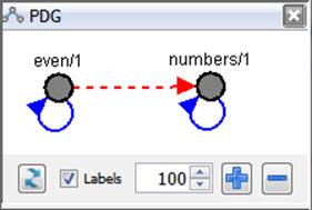
Foreign keys, thus, are useful
devices to specify domain constraints for relations. In contrast to the
relational case, where foreign key constraints can only be applied to tables
(the extensional part of the database), here we admit this also for the
intensional part of the deductive database. A predicate with all their
arguments affected by foreign keys is called here a limited domain predicate.[6]
A limited domain predicate is safe
with respect to negation because its domain is finite whenever its referenced
predicates are also finite. Then, it is possible to submit an open negated call
because the predicate domain is known and the complement of the positive
meaning is thus known as well. For example, the following query is safe and
returns the expected result:
DES> not numbers(X)
Info: Processing:
answer(X) :-
not numbers(X).
{
answer(0),
answer(12),
answer(14),
answer(16),
answer(18),
answer(20)
}
Info: 6 tuples
computed.
The domain of numbers is (0), (2), (4), ... (20) and its positive semantics is defined by the positive program rules as (2), (4), ..., (10). Therefore, the complement of the positive semantics is (0), (12), (14), ..., (20), which is the intended meaning for its negation. Out of curiosity,
let's see the restricted part of the predicate numbers:
DES> -numbers(X)
{
-numbers(1),
-numbers(3),
-numbers(5),
-numbers(7),
-numbers(9)
}
Info: 5 tuples
computed.
It is not possible to submit a
non-ground negated call to this restricted predicate:
DES> not -numbers(X)
Error: not '$p0'(X) might
not be correctly computed because of the unrestricted variable: [X]
Warning: This autoview
is unsafe because of variable: [X]
because the restricting rules has no
limited domain[7]. Still, it is possible to submit ground negated calls as:
DES> not -numbers(0)
Info: Processing:
answer
in the program context of the exploded query:
answer :-
not '$p0'.
'$p0' :-
-numbers(0).
{
answer
}
Info: 1 tuple computed.
DES> not -numbers(1)
Info: Processing:
answer
in the program context of the exploded query:
answer :-
not '$p0'.
'$p0' :-
-numbers(1).
{
}
Info: 0 tuples
computed.
Limited domain predicates are also
useful for hypothetical reasoning, as shown in the next section.
4.1.21 Hypothetical Queries
Hypothetical queries are a common
need in several scenarios, related mainly with business intelligence applications
and the like. They are also known as "what-if" queries and help
managers to take decisions on scenarios which are somewhat changed with respect
to a current state. Such queries are used, for instance, for deciding which
resources must be added, changed or removed to optimize some criterion (cost
function - also well related to optimization technologies). Hypothetical
queries in the database arena are typically used for assumptions w.r.t. a
current database instance.
DES includes one form of Hypothetical
Datalog queries which may serve to answer several questions. The syntax of an
hypothetical query is as follows:
Rule1 /\ ... /\ RuleN => Goal
which means that, assuming that the
current database is augmented with the rules Rule1, ..., RuleN, then Goal is computed with respect to this augmented database (each Rulei must be safe; see Section 5.3). Such a query
is also understood as a literal in the context of a rule, so that any rule can
contain hypothetical goals, as in a :- b => c. In turn, any Rulei can contain hypothetical goals. Variables in Rulei are local to it (i.e., they are neither shared with other rules nor the goal). Moreover,
a hypothetical literal does neither share variables with other literals nor the
head of the rule in which it occurs. Assumed rules can be either regular or
restricting rules.
Borrowing an example from [Bon90][8], we consider an extended and adapted rule-based system for describing
university policy: student(S) means that S is a student, course(C) that C is a course, take(S,C) that student S takes course C, and grad(S) that S is eligible for graduation. The extensional database can contain facts
as:
student(adam).
student(bob).
student(pete).
student(scott).
student(tony).
course(eng).
course(his).
course(lp).
take(adam,eng).
take(pete,his).
take(pete,eng).
take(scott,his).
take(scott,lp).
take(tony,his).
The intensional database can contain
rules as:
grad(S) :- take(S,his), take(S,eng).
A regular query for students that
would be eligible to graduate is:
DES> grad(S)
{
grad(pete)
}
Info: 1 tuple computed.
A first hypothetical query for this
database asks "If Tony took eng, would he be eligible to graduate?", which can be queried with:
DES> take(tony,eng) => grad(tony)
Info: Processing:
answer :-
take(tony,eng)=>grad(tony).
{
answer
}
Info: 1 tuple
computed.
Also, if Pete did not take his, he would not be eligible to graduate (notice the restricting atom, with
a preceding minus sign):
DES> -take(pete,his) => grad(S)
Info: Processing:
answer(S) :-
-(take(pete,his))=>grad(S).
{
}
Info: 0 tuples
computed.
More than one assumption can be
simultaneously stated, as in: "If Tony took eng, and Adam took his, what are the students that are eligible to graduate?"
DES> take(tony,eng) /\ take(adam,his) => grad(S)
Info: Processing:
answer(S) :-
take(tony,eng)/\take(adam,his)=>grad(S).
{
answer(adam),
answer(pete),
answer(tony)
}
Info: 3 tuples
computed.
Another query is "Which are the
students which would be eligible to graduate if his and lp were enough to get it?":
DES> (grad(S) :- take(S,his), take(S,lp)) => grad(S)
Info: Processing:
answer(S) :-
(grad(S):-take(S,his),take(S,lp))=>grad(S).
{
answer(pete),
answer(scott)
}
Info: 2 tuples
computed.
Note that, although S occurs in both the antecedent and the consequent, they are not actually
shared, and they simply act as different variables.
Considering also information about
course prerequisites as:
pre(eng,lp).
pre(hist,eng).
pre(Pre,Post) :-
pre(Pre,X),
pre(X,Post).
One might wonder whether adding a
new prerequisite implies a cycle (so that students cannot fulfil prerequisites
at all for the courses in a cycle):
DES>
pre(lp,hist)=>pre(X,X)
Info: Processing:
answer(X) :-
pre(lp,hist)=>pre(X,X).
{
answer(eng),
answer(hist),
answer(lp)
}
Info: 3 tuples
computed.
The answer includes those nodes in
the graph that are in a cycle (i.e., a course becomes a prerequisite of itself).
Following the example for even
numbers in Section 4.1.19, and given the
regular rule for p is asserted, we can use the following assumption for computing those
numbers:
DES> /assert
p(X) :-
X=1
; p(Y),
Y<10, X=Y+1.
DES>
(-p(X)
:-
p(X),
X mod
2 =
1) =>
p(X)
Info: Processing:
answer(X) :-
(-(p(X)):-p(X),X mod 2=1)=>p(X).
{
answer(2),
answer(4),
answer(6),
answer(8),
answer(10)
}
Info: 5 tuples
computed.
4.1.21.1 Hypothetical Queries and Integrity Constraints
Assumptions can be used in
combination with any of the features of DES; in particular, integrity
constraints. Following the previous example, you can even express it with the
aid of integrity constraints. Avoiding cycles can be forced by:
DES> :-pre(X,X)
Then, if you want to list
prerequisites assuming pre(lp,hist) as before:
DES>
pre(lp,hist)=>pre(X,Y)
Info: Processing:
answer(X,Y) :-
pre(lp,hist)=>pre(X,Y).
Error: Integrity
constraint violation.
ic(X) :-
pre(X,X).
Offending values in database: [ic(lp),ic(eng),ic(hist)]
Info: The following
rule cannot be assumed:
pre(lp,hist).
{
answer(eng,lp),
answer(hist,eng),
answer(hist,lp)
}
Info: 3 tuples
computed.
So, the system informs that there is
an inconsistency when trying to assert such offending fact (pre(lp,hist)), which makes prerequisites to form a cycle (as shown in the offending
value list [ic(lp),ic(eng),ic(hist)]). The system informs about the rules that cannot be assumed but
continues its processing. This is also useful to know the result for the
admissible assumptions. Note that, in general, offending facts can be a subset
of the meaning of an assumed rule in the context of the current database. To
illustrate this, let's consider the following program for throwing a coin:
% Tails win:
:- win, heads.
win :- heads ; tails.
Predicate win states that one wins if either heads or tails are got, and the
constraint states that you have to get tails to win. Then, the following
hypothetical goal states whether assuming heads or tails leads to win.
DES> heads /\ tails => win
Info: Processing:
answer :-
heads/\tails=>win.
Error: Integrity
constraint violation.
ic :-
win,
heads.
Info: The following
rule cannot be assumed:
heads.
{
answer
}
Info: 1 tuple
computed.
As it is informed, heads cannot be assumed in order to win.
4.1.21.2 Hypothetical Queries and Duplicates
win_nim :-
take => one_left.
win_nim :-
take/\take => one_left.
win_nim :-
take => enough, win_nim.
win_nim :-
take/\take => enough, win_nim.
one_left :-
total(N),
count(take,C),
N-C=1.
enough :-
total(N),
count(take,C),
N-C>0.
total(4).
The predicate win_nim states that I win if I take one or
two tokens and there is one left for you. Otherwise, if there are enough tokens
(after taking one or two) to continue playing, then let's see if I can win.
Each occurrence of take in the left hand side of => is an assumed fact that can be
counted if duplicates are enabled (otherwise, the counting will be 0 - if there
is no one - or 1 - if there is one or more, as duplicates are discarded). So,
the predicate one_left determines whether there is exactly
one token left, and enough determines if there is one token
left at least. The predicate total states the total number of tokens
which are available for a game.
For more than 2 tokens there is always both winning and loosing paths
for the player in turn. For exactly 2 tokens there is no loosing path (because
the player cannot take 2 as the heap would be empty). And for 1 token, there is
no winning path:
DES> win_nim
{
}
Info: 0 tuples computed.
Note that enabling duplicates can lead to non-terminating queries. For instance, let's consider:
DES> /duplicates off
DES> /assert p:-p=>p
DES> p
{
p
}
Info: 1 tuple computed.
DES> /duplicates on
DES> p
... Non-terminating
Here, the hypothesis p is recursively added to the
database with no end as there is no terminating condition.
4.1.21.3 Hypothetical Queries and Negation
Implication can also be used in conjunction with negation. Let's
consider the following example, which states flight links (flight/2 for origin and destination)
between airports (airport}), and where flight travels (flight_travel/2 also for origin and destination)
are possible if involved airports are not closed:
flight_travel(X,Y) :-
flight(X,Y),
not closed(X),
not closed(Y).
flight_travel(X,Y) :-
flight_travel(X,Z),
flight_travel(Z,Y).
flight(a,b).
flight(b,c).
flight(c,d).
A regular query for consulting possible travels is:
DES> flight_travel(X,Y)
{
flight_travel(a,b),
flight_travel(a,c),
flight_travel(a,d),
flight_travel(b,c),
flight_travel(b,d),
flight_travel(c,d)
}
Info: 6 tuples computed.
Assuming that airport b is closed, we ask for the possible
travels with this assumption:
DES> closed(b) => flight_travel(X,Y)
Info: Processing:
answer(X,Y) :-
closed(b)=>flight_travel(X,Y).
{
answer(c,d)
}
Info: 1 tuple computed.
where negated calls to closed/1 occur in the first rule of flight_travel/2.
We can also ask for the opposite: Which are the flight travels which are
not possible for that assumption:
DES> flight_travel(X,Y),(closed(b)=>not flight_travel(X,Y))
Info: Processing:
answer(X,Y) :-
flight_travel(X,Y),
closed(b)=>not flight_travel(X,Y).
{
answer(a,b),
answer(a,c),
answer(a,d),
answer(b,c),
answer(b,d)
}
Info: 5 tuples computed.
Note that, first, we ask for all the possible flights (first goal flight_travel(X,Y)) and, then, we restrict to those
flights which are not possible under the assumption. The first goal is needed
for the query to be safe. Recall that Datalog with negation is not constructive
(variables in the negated goal are not instantiated unless their values are
already provided by a positive goal), and answers must be ground. Note, also, that
the meaning of the first occurrence of goal flight_travel(X,Y) in this last query is the very same
as the meaning of the first query. However, the meaning of the second
occurrence of that goal restricts the answer to those flights for which
involved airports are not closed because of the assumption.
Another alternative for such assumption would be to discard those
flights with either its origin or destination at airport b, and then assuming the transitive
closure of the relation flight with travel:
DES> (-flight(X,Y):-flight(X,Y),(X=b;Y=b)) /\
( travel(X,Y):-flight(X,Y);flight(X,Z),travel(Z,Y)) =>
travel(X,Y).
Info: Processing:
answer(X,Y) :-
(-(flight(X,Y)):-flight(X,Y),(X=b;Y=b))/\(travel(X,Y):-flight(X,Y);flight(X,Z),travel(Z,Y))=>travel(X,Y).
{
answer(c,d)
}
Info: 1 tuple computed.
But notice that this is not equivalent to overloading the relation flight with its transitive closure, as
follows:
DES> (-flight(X,Y):-flight(X,Y),(X=b;Y=b)) /\
( flight(X,Y):-flight(X,Y);flight(X,Z),flight(Z,Y)) =>
flight(X,Y).
Info: Processing:
answer(X,Y) :-
(-(flight(X,Y)):-flight(X,Y),(X=b;Y=b))/\(flight(X,Y):-flight(X,Y);flight(X,Z),flight(Z,Y))=>flight(X,Y).
{
answer(a,c),
answer(a,d),
answer(c,d)
}
Info: 3 tuples computed.
Indeed, for computing the meaning of flight, first the meaning of its regular
rules are computed (which deliver its transitive closure including flights
involving airport b), and then, the meaning of its restricting
rules, therefore removing from the transitive closure those flights leaving
from or arriving at airport b.
4.1.22 Fuzzy Datalog
Datalog implements Logic Programming with crisp relations, as opposed to uncertainty as found in some
real-world applications that require approximate
relations. Relations between objects cannot be always precisely specified. As
an example, think of the relations near,
cold, and tall. Usually, in a fuzzy setting they are given an approximation
degree δ for a given pair of related
objects, stating that the first one is related to the second one with
confidence δ.
Fuzzy theory comes as early as [Zade65] and it was applied to logic
programming in the seventies, with the seminal work of R. Char Tung Lee [Lee72].
A relevant work [Sess02] introduces the notion of syntactic similarity and a
weak SLD-resolution for fuzzy logic programs. In DES, we follow the approach of
Bousi~Prolog (BPL) [JR10], which modifies the classical resolution procedure by
replacing the unification algorithm by a fuzzy unification one, based on
proximity relation (a broader kind of binary fuzzy relations that subsumes
similarity relations). In addition, we extend it with approximation degrees for
rules (known as graded rules).
Fuzzy Datalog in DES is a new system mode that must be enabled with the
command:
DES> /system_mode fuzzy
FDES>
which changes the default prompt DES> to FDES>. This command resets the database.
4.1.22.1 Fuzzy Relations and Approximation Degrees
[JR10] defines a proximity/similarity binary relation ~ relating either two predicates or
two function symbols. Here, function symbols are restricted to constant symbols
because DES does not allow user compound terms as data. Fuzzy relations are
extensionally defined by proximity equations, and intensionally by properties
(cf. Section 4.1.22.2). For example, the proximity equation:
so_much ~
very_much = 0.6.
between the constants so_much and very_much states that they are similar with a
degree of 0.6. For this relation, (by default) it is intensionally defined that
a symbol is similar to itself with a degree of 1.0 (reflexivity). Also that very_much ~ so_much = 0.6
(symmetry), cf. Section 4.1.22.2.
By taking an example from that work, let us consider the following
program (in the distribution directory examples/fuzzy/cookies.dl):
% Facts
likes(john, cookies,
a_little).
likes(mary, cookies,
very_much).
likes(peter, cookies,
so_much).
likes(paul, cookies, does_not).
% Rules
buy(X,P) :- likes(X, P,
very_much).
For the query buy(X,cookies) about people prone to buying cookies,
a classical Datalog system (eliding proximity equations) would return the
single answer buy(mary, cookies). However, john and peter are also reasonable candidates to
buy cookies from a real-world interpretation of the relation likes. Hence, if we are looking for a
flexible query answering procedure, more approximate to the real-world setting,
john and peter should appear as answers. So, by
adding the next proximity equations:
% Proximity Equations
relating Constants
does_not ~ a_little
= 0.5.
a_little ~
very_much = 0.2.
does_not ~ so_much = 0.1.
so_much ~
very_much = 0.6.
a_little ~ so_much = 0.4.
then, the query above would return these answers:
FDES> buy(X,cookies)
Info: Processing:
answer(X) :-
buy(X,cookies).
{
answer(mary),
answer(peter)with 0.6,
answer(john)with 0.4,
answer(paul)with 0.4
}
Info: 4 tuples computed.
Any fuzzy query is considered as an autoview (cf. Section 4.1.6), and the answer is built with the relevant
variables in the query. In this example, X is the relevant variable for which
matching values are looked for in the database. Thus, while mary is surely expected to buy cookies
(i.e., with an approximation degree of 1.0 -an approximation degree which is
omitted in the output), both john and paul would buy cookies with an
approximation degree of 0.4, and peter with 0.6 (denoted with the keyword with).
As a second way to state approximation degrees, proximity equations can
be stated between predicates as well. To this end, each predicate symbol in an
equation must be accompanied by its arity. The next example (in the
distribution directory examples/fuzzy/sizes.dl) classifies people on their height
as tall, medium and short, specifying that a medium (resp.
short) person can be understood as a tall (resp. medium) one with a degree of
0.4:
:- t_norm(product).
tall/1
~ medium/1 = 0.4.
medium/1 ~ short/1 = 0.4.
tall(magic_johnson).
tall(paul).
medium(john).
medium(ava).
short(bob).
short(eve).
Looking for tall people, we get:
FDES> tall(X)
Info: Processing:
answer(X) :-
tall(X).
{
answer(magic_johnson),
answer(paul),
answer(ava)with 0.4,
answer(john)with 0.4,
answer(bob)with 0.16,
answer(eve)with 0.16
}
Info: 6 tuples computed.
Notice that the assertion :- t_norm(product) in this program selects a specific
t-norm. A t-norm (represented with the operator D) is the extension of the
first-order logic conjunction for the fuzzy setting, and applies to
approximation degrees. Usual t-norms include: minimum (Göedel), product and Łukasiewicz, where the first one is
the default in DES. Also note that the answer is ordered first by approximation
degree, and then, by tuples.
For the last example, it turns out to be more appropriate a product
t-norm because, by transitivity, if the approximation degree between tall and medium is 0.4, and between medium and short is 0.4, then the approximation
degree between tall and short is computed as 0.4 Dproduct 0.4 = 0.16 (the minimum t-norm
would return 0.4, which does not seem appropriate in this case).
The third and last way to express approximation degrees is for rules in
predicates. Each rule in a predicate may receive a degree to express its
confidence in the context of the predicate. Such rules are known as graded rules. As an example in the stock
market, let us consider the following rules (in the distribution directory examples/fuzzy/stock.dl):
stock_up(google) with 0.9.
stock_up(greek_bonds) with 0.2.
shareholder(paul,google).
shareholder(paul,greek_bonds).
keep_stock(Name,Stock) :-
shareholder(Name,Stock),
stock_up(Stock).
where google stock is expected to raise with a
degree of 0.9 and greek_bonds with 0.2. Then, the query keep_stock(Name,Stock) would return the stocks that are
profitable to keep for each shareholder:
FDES> keep_stock(N,S)
Info: Processing:
answer(N,S) :-
keep_stock(N,S).
{
answer(paul,google)with 0.9,
answer(paul,greek_bonds)with 0.2
}
Info: 2 tuples computed.
In this example, it might be wise to set a degree threshold for the
outcome, which can be done with a l-cut value. For example, we can be
interested in keeping stocks with a degree greater than or equal to 0.8:
FDES> /lambda_cut 0.8
FDES> keep_stock(Name,Stock).
Info: Processing:
answer(N,S) :-
keep_stock(N,S).
{
answer(paul,google)with 0.9
}
Info: 1 tuple computed.
The command /lambda_cut sets this threshold, which can be
alternatively stated in a program as an assertion, with :- lambda_cut(0.8).
Contrary to proximity equations, a graded rule is not overwritten by the
same rule but with a different grade, and the prevailing grade is the maximum
when fuzzy answer subsumption is enabled. For example:
FDES> /assert stock_up(google) with 0.6
FDES> /listing stock_up(google)
stock_up(google) with 0.6.
stock_up(google) with 0.9.
Info: 2 rules listed.
FDES> stock_up(google)
Info: Processing:
answer :-
stock_up(google).
{
answer with 0.9
}
Info: 1 tuple computed.
Both rules are still in the database, as it can be checked by either
listing the rules or disabling fuzzy answer subsumption:
FDES> /listing stock_up(google)
stock_up(google) with 0.6.
stock_up(google) with 0.9.
Info: 2 rules listed.
FDES> /fuzzy_answer_subsumption off
FDES> stock_up(google)
Info: Processing:
answer :-
stock_up(google).
{
answer with 0.9,
answer with 0.6
}
Info: 2 tuples computed.
4.1.22.2 Fuzzy Relations and Properties
A crisp binary relation R
relates values of two domains D1
and D2 as a subset of D1 × D2, so it can be specified as a
characteristic function as well:
![]()
For a binary fuzzy relation R: D × D, this function admits values in the
interval [0,1] and, as classical relations, may enjoy several properties,
including:
· Reflexive: R(x,x) = 1 for all x Î D.
· Symmetric: R(x,y) = R(y,x)
for all x,y Î D.
· Transitive: R(x,z) ≥ R(x,y) D R(y,z) for all x,y,z Î D.
One can extensionally specify fuzzy relations with a set of proximity
equations, and properties that intensionally provide all the tuples in its meaning
(all the entries that define the fuzzy relation). This meaning is computed as a
D-closure (also referred to as
t-closure), which is somewhat similar to a transitive closure by replacing the
conjunction by a t-norm operator D.
Let us consider the following example:
FDES> /abolish
FDES> /assert a~b=0.4
FDES> /assert b~c=0.3
These two proximity equations define the relation ~, which
by default has attached the properties reflexive, symmetric and transitive, and
the t-norm Gödel. The complete meaning of the fuzzy relation can be inspected
with the following command:
FDES> /list_t_closure
a~a=1.0.
a~b=0.4.
a~c=0.3.
b~a=0.4.
b~b=1.0.
b~c=0.3.
c~a=0.3.
c~b=0.3.
c~c=1.0.
Info: 9 equations
listed.
where equations such as a~a=1.0 are deduced by reflexivity, b~a=0.4 by symmetry, and a~c=0.3 by
transitivity. So, users are not obliged to specify the equations that are
intensionally deduced by properties.
Asserting an proximity equation between two symbols for which there is
already another equation results in overwritting the existing equation:
FDES> /abolish
FDES> /assert a~b=0.4
FDES> /assert a~b=0.3
FDES> /list_fuzzy_equations
a~b=0.3.
Info: 1 equation listed.
Typical relations are collected in the following table with respect to
their properties:
|
Relation |
Reflexive |
Symmetric |
Transitive |
|
Strict Order |
no |
no |
yes |
|
Partial Order |
yes |
no |
yes |
|
Proximity |
yes |
yes |
maybe |
|
Similarity |
yes |
yes |
yes |
Properties (reflexive, symmetric and transitive) for the (default) relation ~ can be stated with the command:
/fuzzy_relation ~ [comma-separated property names]
However, the default fuzzy relation ~ is not intended to be modified
because it plays a fundamental role in the so-called weak unification recalled
in next subsection (if changed, unexpected results may occur). Instead, one can
define arbitrary fuzzy relations, as for example the proximity relation near, which can be specified as follows:
/fuzzy_relation near [reflexive,symmetric]
You can specify as many fuzzy relations as needed, which can coexist
with the default ~. We speak of relationship equations
referring to equations of user-defined fuzzy relations. But note that weak
unification only works for this relation.
Properties can be consulted with the same command with no arguments:
FDES> /fuzzy_relation
Info: Properties of '~' are
[reflexive,symmetric,transitive]
As already introduced, the operator D represents the t-norm, where typical
ones and included in DES are:
· Minimum/Göedel (min/goedel): x D y = min(x,y)
· Product (product): x D y =x∙y
· Łukasiewicz (luka/lukasiewicz): x D y = max(0,x+y-1)
· Hamacher Product (hamacher): 
· Nilpotent Minimum (nilpotent): ![]()
These t-norms can be stated and consulted with the command:
/t_norm ~ t-norm_name
As a matter of portability with BPL programs, the t-norm can be stated
in the command /fuzzy_relation as a parameter (between
parentheses) of the transitive property (to this end, also the command synonym /fuzzy_rel is provided). For example:
FDES> /fuzzy_relation ~ [reflexive,symmetric,transitive(product)]
Submitting the goal X~Y in the last example results in
obtaining the whole meaning of the relation ~:
FDES> X~Y
Info: Processing:
answer(X,Y) :-
X~Y.
{
answer(a,a),
answer(b,b),
answer(c,c),
answer(a,b)with 0.4,
answer(b,a)with 0.4,
answer(a,c)with 0.3,
answer(b,c)with 0.3,
answer(c,a)with 0.3,
answer(c,b)with 0.3
}
Info: 9 tuples computed.
Note that this result is valid for a l-cut less or equal to 0.3. If the l-cut value of 0.8 which was
specified in an earlier example remains, then the answer in this case consists
only of the first three answers. If you want to be sure of obtaining the whole
meaning, use the command /list_t_closure instead.
Replacing a variable by any of the constants in the fuzzy relation results
in an appropriate filtering of the relation, as in:
FDES> X~a
Info: Processing:
answer(X) :-
X~a.
{
answer(a),
answer(b)with 0.4,
answer(c)with 0.3
}
Info: 3 tuples computed.
where the outcome shows that the constant a is related to itself with an approximation
degree d of 1.0, with b with d of 0.4, and with c with d of 0.3.
By removing both the reflexive and transitive properties, this goal now
outputs:
FDES> /fuzzy_relation ~ [symmetric]
FDES> X~a
Info: Processing:
answer(X) :-
X~a.
{
answer(b)with 0.4
}
Info: 1 tuple computed.
If the symmetric property would also be removed, no result tuple would
be output in this last query. But recall that unexpected results can occur with
respect to the weak unification and resolution procedures if the default
properties of ~ are changed. So, if other
properties are needed, better define a new fuzzy relation.
4.1.22.3 Weak Unification and Weak Unification Operator
Classical logic programming unification is replaced by weak unification
in which syntactically-different symbols may match with a certain approximation
degree. In Datalog, only constants and variables can be unified because it
implements function-free first-order logic. In the fuzzy setting, two constants
are unifiable is they are similar with an approximation degree greater than or
equal to the current l-cut.
Weak unification implicitly occurs when matching query (or goal)
arguments, as in the following example (taken from Section 4.1.22.1): likes(X,P,very_much). Also, whereas the operator = implements classical (crisp)
equality, the operator ~~ implements an explicit fuzzy weak
unification. The following are examples of explicit weak unification between
Datalog terms (either variables or constants):
FDES> % Next goal delivers an approximation degree 0.4 because it was
specified with a proximity equation
FDES> a~~b
Info: Processing:
answer :-
a~~b.
{
answer with 0.4
}
Info: 1 tuple computed.
FDES> % Due to the reflexive property, the following is true with an
approximation degree 1.0 (which is omitted in the displays)
FDES> a~~a
Info: Processing:
answer :-
a~~a.
{
answer
}
Info: 1 tuple computed.
FDES> % Due to the transitive property, the following is true with an
approximation degree 0.3
FDES> a~~c
Info: Processing:
answer :-
a~~c.
{
answer with 0.3
}
Info: 1 tuple computed.
FDES> % Weak unification provides a representative of unifiers:
FDES> X~~a
Info: Processing:
answer(X) :-
X~~a.
{
answer(a)
}
Info: 1 tuple computed.
Note that the result of a weak unification is a representative of the
class of all possible weak most general unifiers. In the last example, in
addition to X/a with 1, other unifiers include X/b with 0.4 and X/c with 0.3. Notably, the representative is the
best (w.r.t. the computed unification degree) among the possible weak most
general unifiers.
Alternatives for different degrees are only possible for alternative
program rules. For example, given the same proximity equations, we can add the
rules p(a), p(b) and p(c)to the database. Then:
FDES> p(a)
Info: Processing:
answer :-
p(a).
{
answer,
answer with 0.4,
answer with 0.3
}
Info: 3 tuples computed.
4.1.22.4 Fuzzy Expressions
A fuzzy expression Term1 FuzzyRelationOperator Term2 returns the approximation degree
between Term1 and Term2, where FuzzyRelationOperator can be ~ or any other user-defined fuzzy
relation operator. Evaluating a fuzzy expression returns its approximation
degree. Thus, a fuzzy expression can occur at any point in an expression for
which a numeric value is expected. For instance, following the previous
example:
FDES> 1-a~b>0.2
Info: Processing:
answer :-
1-sim(~,a,b)>0.2.
{
answer
}
Info: 1 tuple computed.
4.1.22.5 Accessing Approximation Degrees
By default, approximation degrees are automatically displayed along
answers. They are hidden from the user when, in its compiled form, each goal in
either a conjunctive query or rule body contains an approximation degree. This
degree is internally used to build the outcome approximation degree, as seen in
previous example.[9] Sometimes, it is needed to access
its value to reasoning in terms of it. To this end, we provide the
metapredicate approx_degree/2, which returns in its second
argument the approximation degree of the goal in its first argument.
As an application example, this can be used to emulate a dynamic l-cut in which the computation can
proceed if it is above a (dynamic) value. The following example shows this,
given the same equations as before:
FDES> approx_degree(X~Y,D), D>0.3
Info: Processing:
answer(X,Y,D) :-
approx_degree(X~Y,D),
D>0.3.
{
answer(a,a,1.0),
answer(a,b,0.4),
answer(b,a,0.4),
answer(b,b,1.0),
answer(c,c,1.0)
}
Info: 5 tuples computed.
4.1.22.6 An Application: Recommender Systems
This application is reproduced from [JS18]. Recommender
systems are an effective way to assist people by offering advice on finding
suitable products and services to facilitate online decision-making [CW14]. Subjective
information (such as how a person evaluates a product or service, and how
another person trusts an opinion depending on its confidence) can be specified
with linguistic, fuzzy information. This idea is applied to modelling a small
recommender system for restaurants in Madrid.
We consider people interested in asking
questions relating the location of the restaurant with respect to its own
location, the quality of the restaurant in terms of other's opinions, and the
type of food served. Thus, we can distinguish two fuzzy relations: A proximity
relation near
(reflexive and symmetric) for representing walking distances, and a predefined
similarity relation ~ (which
is, in addition, transitive) for representing quality degrees. These are
defined in the next code excerpt (located in the distribution directory at examples/fuzzy/recommender.dl).
:-fuzzy_relation(near,[reflexive,symmetric]).
sol near callao = 0.6.
sol near cruz = 0.5.
callao near plaza_españa = 0.4.
:-fuzzy_relation(~,[reflexive,symmetric,transitive]).
plain~good=0.5.
good~very_good=0.5.
very_good~excellent=0.3.
The first assertion fuzzy_relation defines
the operator near as a
proximity relation for a walking distance with the reflexive and symmetric
properties. Analogously, a similarity relation ~ is
explicitly defined next (in fact, its assertion can be removed from the program
since it is defined as such by default).
A fuzzy predicate confidence/1
defines the degree of reliability (in the opinion) which a given type of user
deserves. For example, a local guide is assumed to be a person including
serious comments in the database where normal and casual users may not, all of
them with different confidences:
confidence(local_guide) with
0.9.
confidence(normal_user) with 0.5.
confidence(casual_user) with 0.3.
Next, several relations are defined with
facts in the database: The relation restaurant/3
relates the name of a restaurant, its location, and food served. Users and
their types are related in the relation user/3. Finally,
user comments are represented in the relation comment/3
relating user, restaurant, and comment.
restaurant(don_oso,cruz,burguer).
restaurant(rodilla,callao,snacks).
restaurant(roque,sol,rice).
restaurant(tagliatella,benavente,italian).
user(juan,local_guide).
user(sara,normal_user).
user(pepe,casual_user).
comment(juan,don_oso,plain).
comment(juan,rodilla,good).
comment(pepe,roque,excellent).
comment(sara,tagliatella,very_good).
A recommendation relies on the quality of a
restaurant, which is defined with a single rule that takes into account the
comment a user has provided, the type of this user, and its confidence:
quality(Restaurant,Quality)
:-
comment(User,Restaurant,Quality),
user(User,Type),
confidence(Type).
So, in order to provide recommendations, the
rule recommend relates
restaurants (Restaurant) with the
location of the user (Origin),
serving certain food (Food) with an
acknowledged quality (Quality):
recommend(Origin,Food,Quality,Restaurant)
:-
restaurant(Restaurant,Location,Food),
Location near Origin,
quality(Restaurant,Quality).
As an example of a query for this database, the
following system session returns recommendations for a user located at sol:
DES> /system_mode fuzzy
FDES> /consult
recommender
Info: 22 rules consulted.
FDES>
recommend(sol,Food,Quality,Restaurant)
Info: Processing:
answer(Food,Quality,Restaurant)
:-
recommend(sol,Food,Quality,Restaurant).
{ answer(snacks,good,rodilla)with 0.6,
answer(burguer,plain,don_oso)with 0.5,
answer(rice,excellent,roque)with 0.3 }
In this session, after switching the
deductive system to the fuzzy setting, the command /consult loads
the database located in the given file (with default extension .dl). The query returns all possible restaurants
indicating the type of food served, quality and the recommended restaurant. Each
answer tuple is ordered by default with respect to descending approximation
degrees. The first tuple indicates that rodilla has a
support degree of 0.6, which
is a value constructed by taking into account that the restaurant is located at
callao, which
is near sol. Also,
there is a comment from the local guide juan (with a
support of 0.9) stating
that the restaurant is good. The next tuple in the answer set refers to the
restaurant don_oso,
receiving a support degree of 0.5 with
quality plain, because
the same local guide commented on this restaurant with this quality level for a
restaurant located at cruz, near sol. The
last tuple receives a small support because the comment was raised by a user
whose type is scored rather low. We can interactively add information about the
type of the food served with, e.g.:
FDES> /assert
burguer~fast_food=0.7.
FDES> /assert
snacks~fast_food=0.9.
Then, a similar query but looking for good
fast food near sol (with no
need to reload the database) would retrieve:
FDES>
recommend(sol,fast_food,good,Restaurant)
Info: Processing:
answer(Restaurant)
:-
recommend(sol,fast_food,good,Restaurant).
{ answer(rodilla)with 0.6,
answer(don_oso)with 0.5 }
Actually, there are two tuples for don_oso
fulfilling the question, with the same support degree (one for plain and
other for good
quality). Due to the default set-oriented behavior of the system, duplicates
are removed.
Finally, a query for the predicate recommend with
variables in all its arguments would return all possible recommendations. (The
reader is encouraged to try the system with different queries.)
4.1.22.7 Fuzzy Restricted Predicates
The notion of restricted predicates (cf. Section 4.1.19) in the crisp setting can be extrapolated to
the fuzzy setting. While a crisp restricted predicate removes certain tuples
(as defined by the corresponding restricting rules) from its meaning, a fuzzy
restricted predicate lowers the
support of selected tuples as defined by the restricting rules. For example, let
us suppose that we were mostly convinced in the current database that Paula was
brunette, which is a knowledge stated with the fact paula(brunette) with 0.8. But, under another light, we are
not so convinced anymore, and we can add the fact -paula(brunette) with 0.2 (note the minus sign at the
beginning) to lower this perception degree. So:
FDES> /assert paula(brunette) with 0.8
FDES> /assert -paula(brunette) with 0.2
FDES> paula(X)
Info: Processing:
answer(X) :-
paula(X).
{
answer(brunette)with 0.6
}
Info: 1 tuple computed.
Thus, the computed approximation degree for the query results from the
approximation degree of the (positive) predicate minus the approximation degree
of its restricted rules (0.8-0.2 = 0.6 in the example). A result degree
less than or equal to zero for a given tuple leads to rejecting it from the
result. Therefore, using a restricted rule -G (which is equivalent to -G with 1.0) removes all tuples from the
meaning of G.
Restricting rules can be added to both extensional and intensional
predicates. Following the recommender example in Section 4.1.22.6, we want to decrease the confidence
on the quality of don_oso because it seems too high for a
food critic. Then, we can add the rule:
-quality(don_oso,Q) :- quality(Q) with 0.1.
Where the predicate quality/1 simply states the different
qualities (not shown in Section 4.1.22.6, and defined by the rule quality(Q):-comment(_U, _R, Q))[10].
Then, the (computed[11]) quality is accordingly lowered:
FDES> quality(R,Q)
Info: Processing:
answer(Q,R) :-
quality(R,Q).
{
answer(good,rodilla)with 0.9,
answer(plain,don_oso)with 0.8,
answer(excellent,roque)with 0.3
}
Info: 3 tuples computed.
There may be several identical rules (either restricting or not) for the
same predicate with different grades. In this case, the computed approximate
degree of the predicate corresponds to the maximum of the positive meaning
minus the maximum of the negative meaning, as illustrated next:
FDES> /listing stock_up(google)
stock_up(google) with 0.6.
stock_up(google) with 0.9.
Info: 2 rules listed.
FDES> /listing -stock_up(google)
-stock_up(google) with 0.1.
-stock_up(google) with 0.05.
Info: 2 rules listed.
FDES> stock_up(google)
Info: Processing:
answer :-
stock_up(google).
{
answer with 0.8
}
Info: 1 tuple computed.
Usefulness of fuzzy restricted predicates mainly belongs to
decision-making applications, which can be easily modelled with Fuzzy
Hypothetical Datalog, as explained in the next section.
4.1.22.8 Fuzzy Hypothetical Datalog
Assumptions, as in Hypothetical Datalog (c.f. Section 4.1.21), can be stated in Fuzzy Datalog as well. In
this case, not only rules and facts can be assumed, but also graded rules and
proximity equations.
Recalling the example in the stock market (Section 4.1.22.1), let us assume that Paul is willing to buy Amazon
shares with a stock up expectation of 0.7. Then, under this assumption, the
query for determining what stocks are wise to keep returns the following:
FDES> stock_up(amazon) with 0.7 /\ shareholder(paul,amazon) => keep_stock(N,S)
Info: Processing:
answer(N,S) :-
stock_up(amazon) with 0.7
/\
shareholder(paul,amazon)
=>
keep_stock(N,S).
{
answer(paul,google)with 0.9,
answer(paul,amazon)with 0.7,
answer(paul,greek_bonds)with 0.2
}
Info: 3 tuples computed.
As well, we can tune existing information in the database. For example,
the confidence in Greek bonds can be raised:
FDES> stock_up(greek_bonds) with 0.5 => keep_stock(N,S)
Info: Processing:
answer(N,S) :-
stock_up(greek_bonds) with 0.5
=>
keep_stock(N,S).
{
answer(paul,google)with 0.9,
answer(paul,greek_bonds)with 0.5
}
Info: 2 tuples computed.
If we want to test a decreasing confidence in Google, it is not
appropriate to simply assume something as stock_up(google) with 0.6, because there is already a fact (stock_up(google) with 0.9) with higher grade in the database,
a fact that is not overwritten by this assumption. Let us try it:
FDES> stock_up(google) with 0.6 => stock_up(google)
Info: Processing:
answer :-
stock_up(google) with 0.6
=>
stock_up(google).
{
answer with 0.9
}
Info: 1 tuple computed.
Instead, restricted predicates can be used to tune decreasing confidence
grades:
FDES> -stock_up(google) with 0.3 => keep_stock(N,S)
Info: Processing:
answer(N,S) :-
-stock_up(google) with 0.3
=>
keep_stock(N,S).
{
answer(paul,google)with 0.6,
answer(paul,greek_bonds)with 0.2
}
Info: 2 tuples computed.
As expected, the database has not been changed, i.e., the expectations
about Google remain the same after all these assumptions:
FDES> stock_up(google)
Info: Processing:
answer :-
stock_up(google).
{
answer with 0.9
}
Info: 1 tuple computed.
Thus, both fuzzy hypothetical reasoning and restricted predicates makes
it possible to consider a changing scenario for decision-making in this very
tiny and simple stock market example.
As an example of assuming
proximity equations, let us consider a fuzzy relation near that states how
"near" are two cities by train (railways are generally not straight,
and two cities can be connected by a much more train distance than it might been
expected):
:- fuzzy_relation(near,[reflexive,symmetric,transitive(product)]).
madrid
near ciudad_real = 0.6.
ciudad_real near badajoz = 0.4.
badajoz near lisboa = 0.5.
Indeed, the train connection between madrid and badajoz is deceptive, but a new high-speed
rail is under discussion. If built, reaching lisboa would be faster:
FDES> madrid near lisboa
Info: Processing:
answer :-
madrid near lisboa.
{
answer with 0.12
}
Info: 1 tuple computed.
FDES> madrid near badajoz = 0.4 => madrid near lisboa
Info: Processing:
answer :-
madrid near badajoz=0.4
=>
madrid near lisboa.
{
answer with 0.2
}
Info: 1 tuple computed.
In this example, the new (explicit) equation madrid near badajoz = 0.4 has been considered. Before it was,
the link between madrid and badajoz was still available because near is transitive, and its t-closure
included madrid near badajoz = 0.24:
FDES> /list_t_closure near
...
madrid near badajoz=0.24.
...
By recomputing the t-closure of near in the presence of the new explicit
equation, it includes the implicit equation madrid near lisboa = 0.2, which is the one used to compute
the answer.
In addition, it is also possible to replace an existing explicit
equation with an assumption. Recall that only one proximity equation between
two given nodes is allowed in a database (adding a new one overwrites the older
one). So, assuming an existing equation with a different approximation degree
amounts to remove it in the assumption context and add the new equation. Out of
this context, the original equation remains. In the same example, we can just consider
that a new high-speed railway has been built between ciudad_real and badajoz (so that both cities are "closer"):
FDES> ciudad_real near badajoz = 0.6 => madrid near lisboa
Info: Processing:
answer :-
ciudad_real near badajoz=0.6
=>
madrid near lisboa.
{
answer with 0.18
}
Info: 1 tuple computed.
Note that the assumed equation is only applicable in its hypothetical
context, and it has no sense outside:
FDES> (ciudad_real near badajoz = 0.6 => madrid near lisboa), ciudad_real near badajoz = Degree
Info: Processing:
answer(Degree) :-
(ciudad_real near badajoz=0.6
=>
madrid near lisboa),
sim(near,ciudad_real,badajoz)=Degree.
{
answer(0.4)with 0.18
}
Info: 1 tuple computed.
So, the corresponding approximation degree out of such context remains
the same (0.4).
4.1.22.9 Fuzzy Datalog Caveats
Several non-classical Datalog features are not supported, such as:
· Most built-in predicates (such as division, exists, ...)
· Null values (thus neither do outer
joins).
In a nutshell, only expect classical features to work in this fuzzy
setting (in addition to the non-classical ones explicitly described in this
manual).
4.2 SQL
This section describes the main limitations, features, and decisions
taken in adding SQL to DES as a query language, which coexists with Datalog. We
describe four parts of the supported subset of the SQL language: DDL (Data
Definition Language, for defining the database schema), DQL (Data Query
Language, for listing contents of the database) and DML (Data Manipulation
Language, for inserting and deleting tuples)[12], and ISL (Information Schema
Language). Section 4.2.13 resumes the SQL grammar. As ODBC connections
are allowed, some DBMS specific features have been added, as well as features
in ISL which are not covered in the SQL standard.
The syntax recognized by the interpreter is borrowed from the SQL standard.
However, the SQL dialect supported by DES includes features which are not in
this standard, as hypothetical views and the division relational algebra
operator. Section names include the notice (Non-Standard)
to refer to such extra features.
4.2.1 Main Limitations
· No insertions/deletions/updates into
views.
· Strings in displayed outputs are not
enclosed between apostrophes unless they begin with upper case.
· DCL (Data Control Language, for
controlling access rights) is not provided in DES.
4.2.2 Main Features
As main features, we highlight:
· Data query, data definition, data
manipulation, and information schema language parts provided.
· Subqueries (nested queries without
depth limits).
· Correlated queries (tables and
relations in nested subqueries can be referenced by the host query). For
example: SELECT * FROM t,(SELECT a
FROM s)
s WHERE t.a=s.a.
· Subqueries in expressions, as SELECT a
FROM t
WHERE t.a
> (SELECT a
FROM s).
· Table, relation, column, and
expression aliases.
· Support for duplicates and duplicate
elimination (which must be explicitly enabled with the command /duplicates on by contrast to usual DBMS's, in
which this is the default and only one mode).
· Linear, non-linear and mutual recursive
queries (not all current DBMS's support linear queries and no one support
non-linear and mutual recursive ones). In contrast to some current DBMS's,
these queries can be located anywhere a query is allowed.
· Simplified recursive queries are
allowed (Non-Standard): Although
supported, there is no need for using a WITH clause.
· Hypothetical queries (Non-Standard).
· Set operators build relations, which
can be used wherever a data source is expected (FROM clause).
· Null values are supported, along
with outer joins (full, left and right).
· Aggregate functions allowed in
expressions at the projection list and HAVING conditions. GROUP
BY clauses are also allowed.
· View support. Any relation built
with an SQL query can be defined as a view.
· Supported database integrity
constraints include type constraints, existence (nullability), primary keys, candidate
keys, referential integrity, check constraints, functional dependencies (non-standard),
and user-defined constraints.
· Parentheses can be used elsewhere
they are needed and also for easing the reading of statements. Also, they are
not required when they are not needed (in contrast to some current DBMS
systems).
· Suggestions are provided for misspelled
table, view and column names when similar entries are found.
· Type casting is disabled by default.
Enabling this (with /type_casting on) provides the usual behaviour of
current DBMS's allowing, for instance, to insert a string (representing a
number) into a numeric field.
· SQL statements can end with a
semicolon (;) but it is not compulsory unless /multiline on is enabled.
· Any identifier is valid as an user
identifier. For instance, the following statements are valid in DES, but
rejected in most DBMS's.
CREATE TABLE from(from INT, dest INT);
SELECT * FROM from JOIN from using;
Note that using stands for a renaming for the
second from table reference (user identifiers
are shown in lowercase whereas system identifiers are shown in uppercase).
· Syntax error reports for both the
local database and ODBC connections.
· Semantic error reports for the local
database (future work include applying this to external databases).
4.2.3 Datalog vs. SQL
With respect to Datalog, some decisions have been taken:
· As in Datalog, user identifiers are
case-sensitive (table and attribute names, ...). This is not the usual
behaviour of current DBMS's.
· In contrast to Datalog, built-in identifiers
are not case-sensitive. This conforms to the normal behaviour of current DBMS's.
4.2.4 Data Definition Language
This part of the language deals with creating (or replacing), and
dropping tables and views. The schema can be consulted with the command /dbschema.
4.2.4.1 Creating Tables
The first form of this statement is as follows:
CREATE [OR REPLACE] TABLE TableName(Column1 Type1 [ColumnConstraints1], ..., ColumnN
TypeN [ColumnConstraintsN] [, TableConstraints])
This statement defines the table schema with name TableName and column names Column1, ..., ColumnN., with types Type1, ..., TypeN, respectively. If the optional
clause OR REPLACE is used, the table is dropped if
existed already, deleting all of its tuples.
A second form of this statement creates a table with the same schema of
an existing table, following SQL standard optional feature T171:
CREATE TABLE TableName
[(] LIKE ExistingTableName
[)]
This version copies the complete schema, including all integrity
constraints (both predefined and user-defined).
A third, last form of this statement creates a table with a SQL
statement as data and schema generator:
CREATE TABLE TableName
[(] AS SQLStatement
[)]
In this case, a table with name TableName is created with the schema and data
returned by the query SQLStatement.
As indicated by the optional meta-symbols [], parentheses in these two last
forms are not mandatory.
There is provision for several column
constraints:
· NOT
NULL. Existency constraint forbiding null values.
· PRIMARY
KEY. Primary key constraint for only one column.
· UNIQUE. Uniqueness constraint for only one
column (Also allowed the alternative syntax: CANDIDATE
KEY).
· REFERENCES TableName[(Column)]. Referential integrity constraint
for only one column.
· DEFAULT
Expression. Makes the value resulting from
evaluating Expression the value assigned to a column for
which no value is provided in an INSERT statement
· DETERMINED
BY Column. Functional dependency. If this
constraint is applied to the column Column1, then: Column → Column1 (Non-Standard).
· CHECK Condition. Check constraint for columns as in
a WHERE clause.
Also, there is provision for several table
constraints:
· PRIMARY
KEY (Column,...,
Column). Primary key constraint for one or
more columns.
· UNIQUE
(Column,...,
Column). Uniqueness constraint for one or
more columns (Also allowed the non-standard alternative syntax: CANDIDATE
KEY (Column,...,
Column)
· FOREIGN
KEY (Column1,...,
ColumnN)
REFERENCES TableName[(Column1,...,
ColumnN)])].
Referential integrity constraint for one or more columns.
· NOT
NULL Column. Non-standard existence constraint for
Column.
· CHECK
CheckConstraint. Check constraint, as listed next.
Check constraints:
· Condition. As in a WHERE clause
· (ColumnR1,...,
ColumnRN)
DETERMINED BY (ColumnL1,...,
ColumnLN). Functional
dependency: ColumnL1,...,ColumnLN
→ ColumnR1,...,ColumnRN (Non-Standard)
Allowed types include:
· CHAR. Fixed-length string of 1.
· CHAR(n). Fixed-length string of n characters.
· VARCHAR(n) (or VARCHAR2(n) or TEXT(n)). Variable-length string of up to n characters.
· VARCHAR (or STRING). Variable-length string of up to
the maximum length of the underlying Prolog atom.
· INTEGER (or INT or SMALLINT or NUMERIC or DECIMAL). Integer number.
· REAL (or FLOAT). Real number.
· NUMERIC(n)
(or DECIMAL(n)). Integer number of up to n digits.
· NUMERIC(p,s)
(or DECIMAL(p,s)). Decimal number with precision p and scale s.
· DATE. Date (year-month-day).
· TIME. Date (hour:minute:second).
· TIMESTAMP
(or DATETIME). Timestamp (year-month-day
hour:minute:second).
Numeric types rely on the underlying Prolog system (see Section 4.1.18.1). Precision and scale are ignored. Automatic
type casting is disabled by default but can be enabled with /type_casting on to behave similar to SQL systems.
By default, strong typing is applied.
Examples:
CREATE TABLE t(a INT PRIMARY KEY, b STRING)
CREATE OR REPLACE TABLE s(a INT, b INT REFERENCES t(a), PRIMARY KEY (a,b))
Note in this last example that if the column name in the referential
integrity constraint is missing, the referred column of table t is assumed to have the same name
that the column of s where the constraint applies (i.e.,
b). So, an error is thrown because
columns s.b and t.b have different types:
DES> CREATE OR REPLACE TABLE s(a INT, b INT REFERENCES t, PRIMARY KEY (a,b))
Error: Type mismatch s.b:number(int) <> t.b:string(varchar).
Error: Imposing constraints.
A declared primary key or foreign key constraint is checked whenever a
new tuple is added to a table, following relational databases. Recall, first, that
the same database is shared for Datalog and SQL, and second, that asserting production
rules (i.e., those defining the intensional database) from the Datalog side is allowed
but primary key and foreign key constraints are not checked for them (they are
only checked for facts). Then, the following scenario is possible:
DES> create or replace table t(a int, b int, c int, d int, primary key (a,c))
DES> insert into t values(1,2,3,4)
Info: 1 tuple inserted.
DES> % The following is
expected to raise an error:
DES> insert into t values(1,1,3,4)
Error: Primary key violation when trying to insert: t(1,1,3,4)
Info: 0 tuples inserted.
DES> % However, the
following is allowed:
DES> /assert t(X,Y,Z,U) :- X=1,Y=2,Z=3,U=4.
DES> /listing
t(1,2,3,4).
t(X,Y,Z,U) :-
X = 1,
Y = 2,
Z = 3,
U = 4.
A Datalog rule should be viewed as a component of the intensional
database. Current DBMS's avoid to define a view with the same name as a table
and, therefore, there is no way of unexpected behaviours such as the one
illustrated above.
Note that it is possible to have tuples already stored in the database
prior to its corresponding table creation. This means that the CREATE
TABLE statement can fail if any of those tuples does not meet all the
constraints stated for the table. For instance, let's consider:
DES> /assert t(null)
DES> create table t(a int primary key)
Error: Null values found for t.[a]
Offending values in database: [nn($NULL(0))]
Info: Constraint has not been asserted.
DES> /dbschema
Info: Database '$des'
Info: No tables.
Info: No views.
Info: No integrity constraints.
Next, a very simple example is reproduced to illustrate basic constraint
handling:
DES> create or replace table u(b int primary key,c int)
DES> create or replace table s(a int,b int, primary key (a,b))
DES> create or replace table t(a int,b int,c int,d int, primary key (a,c), foreign key (b,d) references s(a,b), foreign key(b) references u(b))
DES> insert into t values(1,2,3,4)
Error: Foreign key violation t.[b,d]->s.[a,b] when trying to insert:
t(1,2,3,4)
Info: 0 tuples inserted.
DES> insert into s values(2,4)
Info: 1 tuple inserted.
DES> insert into t values(1,2,3,4)
Error: Foreign key violation t.[b]->u.[b] when trying to insert:
t(1,2,3,4)
Info: 0 tuples inserted.
DES> insert into u values(2,2)
Info: 1 tuple inserted.
DES> insert into t values(1,2,3,4)
Info: 1 tuple inserted.
DES> /listing
s(2,4).
t(1,2,3,4).
u(2,2).
4.2.4.2 Creating Views
CREATE [OR REPLACE] VIEW ViewName[(Column1, ..., ColumnN)]
AS SQLStatement
This statement defines the view schema in a similar way as defining
tables. The view is created with the SQL statement SQLStatement as its definition. If the optional
clause OR REPLACE is used, the view is firstly dropped
if existed already. Other tuples or rules asserted (with the command /assert) are not deleted, as the next
example shows:
DES> /assert v(1)
DES> create or replace view v(a) as select 2
DES> select * from v
answer(v.a:int) ->
{
answer(1),
answer(2)
}
Info: 2 tuples computed.
Note that column names are not mandatory.
Examples:
DES> CREATE VIEW v(a,b,c,d) AS
SELECT * FROM t WHERE a>1;
DES> CREATE OR REPLACE VIEW w(a,b) AS
SELECT t.a,s.b FROM t,s WHERE t.a>s.a;
DES> /dbschema
Info: Table(s):
* s(a:int,b:int)
- PK: [a,b]
* u(b:int,c:int)
- PK: [b]
* t(a:int,b:int,c:int,d:int)
- PK: [a,c]
- FK: t.[b,d] -> s.[a,b]
- FK: t.[b] -> u.[b]
Info: View(s):
* v(a:int,b:int,c:int,d:int)
- Defining SQL Statement:
SELECT ALL *
FROM
t
WHERE a > 1;
- Datalog equivalent rules:
v(A,B,C,D) :-
t(A,B,C,D),
A > 1.
* w(a:int,b:int)
- Defining SQL Statement:
SELECT ALL t.a, s.b
FROM
t,
s
WHERE t.a > s.a;
- Datalog equivalent rules:
w(A,B) :-
t(A,C,D,E),
s(F,B),
A > F.
Info: No integrity constraints.
Note that primary key constraints follow the table schema, and inferred
types are in the view schema.
4.2.4.3 Dropping Tables
DROP TABLE OptionalClauses
TableName OptionalClauses
This statement drops the table schema corresponding to TableName, deleting all of its tuples
(whether they were inserted with INSERT or with the command /assert) and rules (which might have been
added via /assert). Any referential integrity
constraint pointing to TableName is dropped. OptionalClauses includes IF
EXISTS and CASCADE. If the clause IF
EXISTS is included, dropping an inexistent table does not raise an error. If
the clause CASCADE is included, dropping a table
implies dropping all views depending on TableName.
Example:
DROP TABLE t
See also:
· Command for dropping all tables
(Section 5.17.1): /drop_all_tables
· Command for dropping all relations
(Section 5.17.1): /drop_all_relations
4.2.4.4 Dropping Views
DROP VIEW OptionalClauses
ViewName OptionalClauses
This statement drops the view with name ViewName, deleting all of its tuples (inserted
with the command /assert) and rules (which might have been
added via /assert). OptionalClauses includes IF
EXISTS and CASCADE. If the clause IF
EXISTS is included, dropping an inexistent view does not raise an error. If
the clause CASCADE is included, dropping a view
implies dropping all views depending on ViewName.
Example:
DROP VIEW v
See also:
·
Command
for dropping all views (Section 5.17.1): /drop_all_views
· Command for dropping all relations
(Section 5.17.1): /drop_all_relations
4.2.4.5 Renaming Tables
RENAME TABLE TableName
TO NewTableName
This non-standard statement (following IBM DB2) allows to change the
name of table TableName to NewTableName. Foreign keys referring to this
table are modified accordingly. Also, views including referenes to this table
are modified to refer to the new name.
4.2.4.6 Renaming Views
RENAME VIEW ViewName
TO NewViewName
This non-standard statement (following IBM DB2) allows changing the name
of view ViewName to NewViewName. Also, views including references
to this view are modified to refer to the new name.
4.2.4.7 Modifying Tables
There are three main ways for modifying (altering) a table: either
adding/dropping constraints, or renaming a column, or redefining a column (both
its data type and constraints), or only changing its data type. The last two
are not in the SQL standard.
The first alternative is:
ALTER TABLE TableName
[ADD|DROP] CONSTRAINT TableConstraint
This statement allows adding and dropping constraints. Syntax of TableConstraint is as of table constraints, where a
constraint specification is expected (instead of a constraint name).
For instance:
DES> create table t(a int primary key check(a>0))
DES> /dbschema
Info: Database '$des'
Info: Table(s):
* t(a:int)
- PK: [a]
- IC:
+ SQL Check:
a > 0
+ Datalog Check:
'$ic_t0'(A) :-
t(A),
A=<0.
Info: No views.
Info: No integrity constraints.
DES> alter table t drop constraint primary key
Error: (SQL) Expected sequence of column names between parentheses after
'alter table t drop constraint primary key'.
DES> alter table t drop constraint primary key(a)
DES> /development on
DES> /dbschema
Info: Database '$des'
Info: Table(s):
* t(a:int)
- IC:
+ SQL Check:
a > 0
+ Datalog Check:
'$ic_t0'(A) :-
t(A),
A=<0.
Info: No views.
Info: No integrity constraints.
DES> alter table t drop constraint check(a>0)
DES> /dbschema
Info: Database '$des'
Info: Table(s):
* t(a:int)
Info: No views.
Info: No integrity constraints.
Note here that a column constraint as primary
key is not allowed, and the equivalent table constraint must be used
instead.
The second alternative is:
ALTER TABLE TableName
RENAME COLUMN OldColumn
TO NewColumn
This statement renames the column with name OldColumn to NewColumn. Any constraints referring to this
column is updated. The following example shows this:
DES> create or replace table t(a int references s default 0, b int, c int determined by a, primary key (a,b), check a+c<10)
DES> /dbschema
Info: Database '$des'
Info: Table(s):
* s(a:int)
- PK: [a]
* t(a:int,b:int,c:int)
- PK: [a,b]
- FK: t.[a] -> s.[a]
- DE: a <- 0
- FD: [a] -> [c]
- IC:
a + c < 10
Info: No views.
Info: No integrity constraints.
DES> alter table t rename column a to d
DES> /dbschema
Info: Database '$des'
Info: Table(s):
* s(a:int)
- PK: [a]
* t(d:int,b:int,c:int)
- PK: [d,b]
- FK: t.[d] -> s.[a]
- DE: d <- 0
- FD: [d] -> [c]
- IC:
d + c < 10
Info: No views.
Info: No integrity constraints.
The third alternative is:
ALTER TABLE TableName
ALTER [COLUMN] Column Type [ColumnConstraints]
This statement redefines Column with data type Type and constraints ColumnConstraints (if provided). Any existing
constraint referring to this column is removed (even table constraints). If
table data can be kept for the new column definition, executing this statement
succeeds. Otherwise, its execution is rejected. The following example shows
this:
DES> create table t(a int primary key, b string, check (a>0))
DES> alter table t alter column a string default ''
DES> /describe t
Info: Database '$des'
Info: Table:
* t(b:string,a:string)
- DE: a <- ''
Note that both the column and table constraints are removed, and only
the new default constraint remains. Further, any other foreign key constraint
referencing the altered table will be removed:
DES> /dbschema
Info: Database '$des'
Info: Table(s):
* s(a:int)
- FK: s.[a] -> t.[a]
* t(a:int,b:string)
- PK: [a]
Info: No views.
Info: No integrity constraints.
DES> alter table t alter column a string default ''
DES> /dbschema
Info: Database '$des'
Info: Table(s):
* s(a:int)
* t(a:string,b:string)
- DE: a <- ''
Info: No views.
Info: No integrity constraints.
Whether existing data can be kept depends on the current type casting
setting: If enabled (with the command /type_casting on), more opportunities of keeping
data are expected. For example:
DES> create table t(a int primary key, b string, check (a>0))
DES> insert into t values(1,'a')
Info: 2 tuples inserted.
DES> alter table t alter column a string default ''
Error: Type mismatch $_t.a:string(varchar) vs. number(integer).
$_t(a:string(varchar),b:string(varchar)) (declared types).
Info: 0 tuples inserted.
DES> /type_casting on
DES> alter table t alter column a string default ''
Info: 1 tuple inserted.
DES> select * from t
answer(t.a:string,t.b:string) ->
{
answer('1',a)
}
Info: 1 tuple computed.
Finally, the fourth alternative is:
ALTER TABLE TableName
ALTER [COLUMN] Column SET [DATA] TYPE Type
This alternative is almost equivalent to the second one by specifying
only the data type. As a difference, existing constraints are not removed. For
example:
DES> create table t(a int primary key determined by b, b string default '', check (a>0))
DES> alter table t alter column b set data type varchar(10)
DES> /describe t
Info:
Database '$des'
Info: Table:
* t(a:int,b:varchar(10))
- PK: [a]
- DE: b <- ''
- FD: [b] -> [a]
- IC:
a > 0
4.2.4.8 Dropping Databases
DROP DATABASE
This statement drops the current database, dropping all tables, views,
and rules (this includes Datalog rules and constraints that may have been
asserted or consulted). It behaves exactly as the command /abolish except that it asks for user
confirmation.
Example:
DES> drop database
Info: This will drop all views, tables, constraints
and Datalog rules.
Do you want to proceed? (y/n) [n]:
4.2.5 Data Manipulation Language
This part of the language deals with inserting, deleting and updating tuples
in tables. SQL insertions, deletions and updates are not allowed for views.
4.2.5.1 Inserting Tuples
There are two forms of inserting tuples. The first one explicitly states
what tuples are to be inserted:
INSERT INTO TableName[(Col1,…,ColN)] VALUES (Expr1,...,ExprN) [, ..., (Expr1,...,ExprN)]
This statement inserts into the table TableName as many tuples as those built with each
tuple of expressions Expr1, ..., ExprN, and Col1 to ColN are non-repeated column names of
the table. Expressions are evaluated before inserting the tuple. If no column
names are given, N is expected to be the number of
columns of the table. If column names are given, each expression Expri corresponds to column name Coli. For those column names which are
not provided in a column name sequence, nulls are inserted. The keyword DEFAULT can be used instead of a constant
(this makes to select either null or the value defined with the DEFAULT constraint in the CREATE TABLE statement).
The next example inserts a single tuple:
CREATE TABLE t(a int, b int DEFAULT 0)
INSERT INTO t VALUES (1,1)
The next one inserts a single tuple into the same table (automatically applying
a null value for the non-provided column a):
INSERT INTO t(b) VALUES (2)
Which is equivalent to:
INSERT INTO t(b,a) VALUES (2,null)
and represents the tuple (null,2). Note that the order of provided
column names represent the order of corresponding values; in this example, the
columns are reversed with respect to the table definition.
For inserting several tuples at a time:
INSERT INTO t VALUES (1,1),(null,2)
The default value defined for the column b can be used in these two sentences:
INSERT INTO t(a) VALUES (1)
INSERT INTO t(a,b) VALUES (2,DEFAULT)
The first one inserts the tuple (1,0), and the second one the tuple (2,0).
Default values for all columns can be expressed as in:
INSERT INTO t DEFAULT VALUES
Expressions for default values can be used instead of just values in the
table definition. For instance:
DES> CREATE TABLE t(a int, b time DEFAULT CURRENT_TIME+30)
DES> INSERT INTO t(a) VALUES (1)
Info: 1 tuple inserted.
DES> SELECT CURRENT_TIME
answer($a0:datetime(time)) ->
{
answer(time(19,44,20))
}
Info: 1 tuple computed.
DES> SELECT * FROM t
answer(t.a:int,t.b:datetime(time)) ->
{
answer(1,time(19,44,50))
}
Info: 1 tuple computed.
It is possible to specify expressions instead of values when inserting
tuples, as:
INSERT INTO t(a) VALUES (sqrt(5)^2);
The second form of the INSERT statement allows to inserting
tuples which are the result of a SELECT statement:
INSERT INTO TableName[(Col1,…,ColN)] SQLStatement
This statement inserts into the table TableName as many tuples as returned by the
SQL statement SQLStatement. This statement has to return as
many columns as either the columns of TableName, if no column names are given, or
the number of provided column names (N), otherwise.
Examples:
INSERT INTO t SELECT * FROM s
You can also insert tuples into a table coming directly (or indirectly)
from the table itself for duplicating rows, as in:
INSERT INTO t SELECT * FROM t
Note that there is no recursion in this query as the source table t is not changed during solving the SELECT statement.
For testing the new (duplicated) contents of t, you can use /listing
t, instead of a SELECT statement, since this statement
always returns a set (no duplicates) when duplicates are disabled (cf. Section 4.1.9).
As in the first form, you can specify columns of the target table as in:
INSERT INTO t(b) SELECT a FROM t
which inserts as many rows in t as it had before insertion, and for each
row, a new tuple is built with the value of the source column a in the target column b, and null in the target column a.
4.2.5.2 Deleting Tuples
DELETE FROM TableName
[[AS] Identifier] [WHERE Condition]
This statement deletes all the tuples of the table TableName that fulfil Condition. It does not delete production rules
asserted via /assert.
Examples:
DELETE FROM t
which deletes all tuples from table t.
DELETE FROM t WHERE a>0
which only deletes tuples from the table t such that the value for the column a is greater than 0.
Aliases can be used in correlated subqueries, as in:
DELETE FROM Contracts C
WHERE NOT EXISTS (SELECT *
FROM Contains
WHERE Reference = C.Reference);
4.2.5.3 Updating Tuples
UPDATE TableName
[[AS] Identifier] SET Att1=Expr1,...,AttN=ExprN [WHERE Condition]
This statement updates each column Atti with the values computed for each Expri for all the tuples of the table TableName that fulfil Condition.
Example:
UPDATE Employees SET Salary=Salary*1.1 WHERE Id IN
(SELECT Id from Promoted WHERE Year='2026');
which increases in a 10% the salaries of the employees which have been promoted
in 2026.
4.2.6 Data Query Language
There are three main types of SQL query statements: SELECT statements, set statements (UNION, INTERSECT, and EXCEPT), and WITH statements (for building recursive
queries).
4.2.6.1 Basic SQL Queries
The syntax of the basic SQL query statement is:
SELECT [DISTINCT|ALL] ProjectionList
[FROM Relations
[WHERE Condition]
[ORDER BY OrdExpressions]
]
Where:
· Square brackets indicate that the
enclosed text is optional. Also, the vertical bar is used to denote alternatives.
· ProjectionList is a list of comma-separated
columns or expressions that will be returned as a tuple result. Wildcards are
allowed, as * (for referring to all the columns
in the data source) and Relation.* (for referring to all the columns in
the relation Relation). The name Relation can be the name of a table, view or
an alias (for a table or subquery). The clause DISTINCT discards duplicates whereas the clause
ALL does not (this is only noticeable
when duplicates are enabled with the command /duplicates on).
· Condition is a logical condition built from
comparison operators (=, <>, !=, <, >, >=, and <=), Boolean operators (AND, OR, XOR, and NOT), Boolean constants (TRUE, FALSE), the existence operator (EXISTS) and the membership operator (IN). See the grammar description in Section
4.2.13 for details. Subqueries are allowed with no
limitations.
· Relations is a list of comma-separated
relations. A relation can be either a table name, or a view name, or a
subquery, or a join relation. They can be renamed via aliases. If no FROM clause is provided, the built-in DUAL relation is used as a data source
(cf. Section 4.2.6.1.2).
· OrdExpressions is a list of comma-separated
ordering expressions. An ordering expression can be either simply an expression
or an expression followed by the ordering criterion (ASC -or ASCENDING- for ascending order, and DESC -or DESCENDING- for descending order). Answers are
ordered by default (see /order_answer) but this order is overridden if
the ORDER BY clause is either directly used in a
query or in the definition of a view the query refers to. The order is based on
the standard order of terms of the underlying Prolog system (see Section 0). An ordering expression can include both an
alias as defined in ProjectionList and aggregate functions. Positional
notation (such as in DB2 and PostgreSQL) is also allowed (though its use is
commonly discouraged).
Examples:
Given the tables:
CREATE TABLE s(a int, b int);
CREATE TABLE t(a int, b int);
CREATE TABLE v(a int, b int);
We can submit the following queries:
SELECT distinct a
FROM t
SELECT t.*, s.b
FROM t,s,v
WHERE t.a=s.a AND v.b=t.b
SELECT t.a, s.b, t.a+s.b
FROM t,s
WHERE t.a=s.a
SELECT *
FROM (SELECT * from t) as r1,
(SELECT * from s) as r2
WHERE r1.a=r2.b;
SELECT *
FROM s
WHERE s.a NOT IN SELECT a FROM t;
SELECT *
FROM s
WHERE EXISTS
SELECT a
FROM t
WHERE t.a=s.a;
SELECT *
FROM s
WHERE s.a > (SELECT a FROM t);
SELECT 1, a1+a2, a+1 AS a1, a+2 AS a2
FROM t;
SELECT 1;
SELECT a FROM t ORDER BY -a;
SELECT CAST(MONTH(CURRENT_DATE) AS STRING) || ' - ' || CAST(YEAR(CURRENT_DATE) AS STRING);
Notes:
· SQL expressions follow the same
syntax as Datalog.
· An SQL expression can be renamed and
used in other expressions.
· Circular definitions will yield
exceptions at run-time, as in a+a3 AS a3
· Terms in expressions in the select
list are first tried as built-in constants and functions. This may lead to
confusion. For example:, creating a table with a column with name e, and selecting e from this table renders:
DES> CREATE TABLE t(e int);
DES> INSERT INTO t VALUES (1);
Info: 1 tuple inserted.
DES> SELECT e FROM t;
answer($a1:float) ->
{
answer(2.718281828459045)
}
Info: 1 tuple computed.
That is, e represents the Euler arithmetic
constant, and in this query, its numerical value is returned. If you want to
access the column name e, then use qualification, as
follows:
DES> SELECT t.e FROM t;
answer(t.e:int) ->
{
answer(1)
}
Info: 1 tuple computed.
A join relation is either of the form:
Relation NATURAL JoinOp
Relation
or:
Relation JoinOp
Relation [JoinCondition]
where Relation is as before (without any
limitation), JoinOp is any join operator (including [INNER]
JOIN, LEFT [OUTER]
JOIN, RIGHT [OUTER]
JOIN, and FULL [OUTER]
JOIN), and JoinCondition can be either:
ON Condition
or:
USING (Column1,...,ColumnN)
where Condition is as described in the WHERE clause, and Column1, ..., ColumnN are common column names of the
joined relations. Omitting the condition in a non-natural join is equivalent to
a true condition. Note that the clause USING does not apply to NATURAL joins, but like them, arguments for
the equijoin occur only once in the result.
Examples:
Given the tables:
CREATE TABLE s(a int, b int);
CREATE TABLE t(a int, b int);
CREATE TABLE v(a int, b int);
We can submit the following queries:
SELECT *
FROM t INNER JOIN s ON t.a=s.a AND t.b=s.b;
SELECT *
FROM t NATURAL INNER JOIN s;
SELECT *
FROM t INNER JOIN s USING (a,b);
SELECT * FROM t INNER JOIN s USING (a);
SELECT *
FROM t INNER JOIN s USING (b);
SELECT *
FROM (t INNER JOIN s ON t.a=s.a) AS s, v
WHERE s.a=v.a;
SELECT *
FROM (t LEFT JOIN s ON t.a=s.a) RIGHT JOIN v ON t.a=v.a;
SELECT * FROM t FULL JOIN s ON t.a=s.a;
Notes:
- The default keyword ALL following SELECT retains duplicates whenever
duplicates are enabled (command /duplicates on). In turn, DISTINCT discards duplicates. But note that
if duplicates are disabled, both ALL and DISTINCT behave the same (i.e., discarding
duplicates).
- The column list for USING must be enclosed between
parentheses; otherwise, the name USING can be used as an alias.
4.2.6.1.1 Top-N Queries
The number of computed tuples for a select statement can be limited with
the so-called Top-N queries. ISO 2008 includes this as a final clause in the SELECT statement:
SELECT [DISTINCT|ALL] ProjectionList
FROM Rels
…
FETCH FIRST Integer ROWS ONLY
However, DES also provides another non-standard, but common form in
other RDBMS's of such queries:
SELECT [TOP Integer] [DISTINCT|ALL] ProjectionList
…
You can switch the order of the TOP and DISTINCT clauses, and even the weird case of
simultaneously specifying both forms of Top-N queries in the same statement, as
long as they express the same limit.
Results of top-N queries may not follow the order in which tuples were
asserted in the database, because their processing depends on the tabled
deductive engine, which keeps results from former computations.
4.2.6.1.2 The dual table
The dual table is a special one-row, one-column
table present by default in Oracle databases. It is suitable for computing
expressions and selecting a pseudo column with no data source. As propositional
relations are also allowed in DES, dual does not need a column at all, and
it is therefore defined as a single fact without arguments. This table can be
used to compute arithmetic expressions as, e.g.:
DES> select sqrt(2) from dual
answer($a0:float) ->
{
answer(1.4142135623730951)
}
Info: 1 tuple computed.
As in MySQL, DES also allows to
omit the FROM clause in theses cases (the
compilation from SQL to Datalog adds the dual table as data source):
DES> select sqrt(2)
answer($a0:float) ->
{
answer(1.4142135623730951)
}
Info: 1 tuple
computed.
Although this table is not displayed with the
command /dbschema, it can be nevertheless dropped with a DROP TABLE SQL statement. If it is deleted, the just described behaviour is no
longer possible. In addition, it cannot be re-declared with a CREATE TABLE SQL statement, but with a type declaration, as :-type(dual). Both the statement DROP DATABASE and the command /abolish restore this table.
4.2.6.2 A More Developed SQL Query Description
The syntax of the basic SQL query
statement is:
SELECT [TOP Integer] [[ALL|DISTINCT]] ProjectionList
[INTO TargetList]
[FROM Relations
[WHERE WhereCondition]
[GROUP BY GroupExpressions]
[HAVING HavingCondition]
[ORDER BY OrderDescription]
[OFFSET Integer [LIMIT Integer]]
[FETCH FIRST Integer ROWS ONLY]]
Where:
· SelectTargetList is the list of comma-separated system/user variable names which receives
the values from ProjectionList. This allows to communicate SQL return values with the basic
scripting system. For example, SELECT 1 INTO v stores the number 1 in the user variable v. Note that the other way round of communication is by including variables
surrounded by $ signs for injecting values from the scripting system to SQL (as, e.g., SELECT * FROM t WHERE a=$v$, where v is a variable defined with the command /set).
· TOP N selects the first N returned rows from the query.
· GROUP
BY groups tuples by the criterion
specified by GroupExpressions
· HAVING applies a condition on groups.
· OFFSET returns a number of tuples (those specified by LIMIT or all otherwise) starting at a given displacement (0 for the first
tuple).
· FETCH behaves as TOP, and both can be used in recursive definitions.
Refer to Section 4.2.13 to inspect the
full SQL grammar supported by DES.
4.2.6.2.1 TOP, OFFSET, LIMIT and FETCH
The following query limits the
result set to the first n computed rows:
select
top
n ... from ...
and is equivalent to the following
others:
select ... from ... offset 0 limit
n
select ... from ... limit
n
select ... from ... fetch first
n rows only
These are alternative syntactic
forms to support the syntax of different SQL systems.
Note that setting n to 0 produces no rows and the system warns about it as in:
DES> select top 0 'Test' from dual
Warning: [Sem]
LIMIT/TOP 0 returns nothing.
Warning: [Sem]
Inconsistent condition.
answer($a0:string) ->
{
}
Info: 0 tuples
computed.
The system also warns for a 0-offset,
which does nothing, as in:
DES> select 'Test' from dual offset 0
Warning: [Sem] OFFSET
0 does nothing.
answer($a0:string) ->
{
answer('Test')
}
Info: 1 tuple
computed.
Imposing an offset implies to add a
stratum; so, a view with an offset cannot be part of a recursive cycle (unless
a 0-offset).
4.2.7 String Operations
This section lists string predicates
and functions which can be used for testing strings and building string
expressions, respectively.
4.2.7.1 CONCAT (Non-ISO)
The function concat(String1, String2) returns a string as the concatenation of String1 and String2. The infix operators || (ISO) and + (Non-ISO) can also be used to concatenate strings.
4.2.7.2 INSTR (Non-ISO)
The function instr(String,
Substring) return the first numeric position (1 base index) in String of the searched Substring.
4.2.7.3 LENGTH (Non-ISO)
The function length(String) returns the number of characters of String.
4.2.7.4 LIKE (ISO)
The predicate like is used for pattern matching on strings, where patterns are built with
constants and two special characters:
- Percent (%), which matches any substring.
- Underscore (_), which matches any character.
Patterns are case sensitive. The
following example retrieves the employees whose names start with 'N':
DES> select employee from works where employee like 'N%'
answer(works.employee:string) ->
{
answer('Nolan'),
answer('Norton')
}
Info: 2 tuples
computed.
It is possible to provide an escape
character should the pattern must include one of the special character. For
example, the next query retrieves e-mail addresses containing at least one
underscore:
DES> select email from employees where email like '%_%' escape '_'
answer(employees.email:string) ->
{
answer('a_nolan@gmail.com')
}
Info: 1 tuple computed.
Values, patterns and the escape
character can be formed as expressions involving constants, columns, and other
string operations.
4.2.7.5 LOWER (ISO)
The function lower(String) returns the lower case version of String.
4.2.7.6 LPAD (Non-ISO)
The function lpad(String, Width [, Fill]) appends either spaces or Fill (if specified) to the left of String for a total width Width.
4.2.7.7 LTRIM (Non-ISO)
The function ltrim(String) removes leading spaces from String.
4.2.7.8 REPLACE (Non-ISO)
The function replace(String, Find,
Replace) replaces the string Find by Replace in the given string String.
4.2.7.9 REVERSE (Non-ISO)
The function reverse(String) reverses the string String.
4.2.7.10 RPAD (Non-ISO)
The function rpad(String, Number [, Fill])
appends either spaces or Fill (if specified) to the right of String for a total width Width.
4.2.7.11 RTRIM (Non-ISO)
The function rtrim(String) removes trailing spaces from String.
4.2.7.12 SUBSTR (Non-ISO)
The function substr(String, Offset [, Length]) returns a string that consists of Length characters from String starting at the Offset position. An offset ranges from 1 (first position of the string) up to
the length of the string. An offset greater than this length makes the result
to be an empty string. As well, an empty string is returned for a length less
than 1. If Offset is negative and Length is greater than -Offset, then the first Length+Offset+1
characters are returned (up to the
length of the string).
If Length is not provided, it returns all the string characters starting at
the Offset position.
4.2.7.13 TRIM (Non-ISO)
The function trim(String) removes both leading and trailing spaces from String.
4.2.7.14 UPPER (ISO)
The function upper(String) returns the upper case version of String.
4.2.8 Conversion Functions
SQL is a strong typed language (to
an extent). Thus, it provides several functions to convert data from one type
to another.
4.2.8.1 EXTRACT (ISO)
The function extract(field
from
datetime) extracts the given field (year, month, day, hour, minute, or second) from a datetime value (date, time or timestamp/datetime). See also Section 4.7.6 for functions
extracting parts of a datetime type.
4.2.8.2 CAST (ISO)
The function cast(value as type) converts the data value to a type type. It can be used with the alternative syntax cast(value,type).
4.2.8.3 TO_CHAR (Non-ISO)
The function to_char(Datetime [, Format]) converts a Datetime to a string for the given Format if specified; otherwise, the current date and time formats are assumed.
4.2.8.4 TO_DATE (Non-ISO)
The function to_date(String [, Format]) converts a String to a datetime for the given Format if specified; otherwise, the current date and time formats are assumed.
4.2.8.5 ASC (Non-ISO)
The function asc(String)returns the ASCII code from a character String.
4.2.8.6 CHR (Non-ISO)
The function chr(Integer)returns the character from an ASCII code Integer.
4.2.8.7 Automatic Type Casting
By enabling automatic type casting
with the command /type_casting on, similar results to current DBMS are got. DES
tries to convert to the more general type when solving SQL queries. For
example:
DES> create table t(a date, b varchar(10))
DES> insert into t values('2020-01-01','2020-01-01')
DES> select * from t where a=b
answer(t.a:datetime(date),t.b:varchar(10)) ->
{
answer('2020-01-01','2020-01-01')
}
Info: 1 tuple
computed.
However, systems such as PostgreSQL
returns an error in this case:
DES> select * from t where a=b
Error: ODBC Code 1: ERROR:
operator does not exist: date = character varying;
Error while executing the query
4.2.9 (Multi)Set Expressions (Non-Standard)
Expressions in the projection list
and conditions (in having and where clauses) are scalar following the standard.
However, DES allows non-scalar expressions dealing to multisets (sets, if
duplicates are disabled as by default).
In the following example, the table t will contain values 1 and 2 for its single field a. By selecting the sum of a from two instances of t, we get the different summations (1+1, 1+2, 2+1, and 2+2):
DES> create table t(a int)
DES> insert into t values (1),(2)
Info: 2 tuples
inserted.
DES> select (select a from t)+(select a from t) from dual
answer($a4:int) ->
{
answer(2),
answer(3),
answer(4)
}
Info: 3 tuples
computed.
DES> /duplicates on
DES> select (select a from t)+(select a from t) from dual
answer($a4:int) ->
{
answer(2),
answer(3),
answer(3),
answer(4)
}
Info: 4 tuples
computed.
If the multiset expression is
located at a condition, this condition is examined for each value of the
expression, giving as many alternatives as true condition instances:
DES> select 1 from dual where (select a from t)>0
answer($a2:int) ->
{
answer(1),
answer(1)
}
Info: 2 tuples
computed.
In this example, following the
previous one, there are two values for a in t that makes true the select condition. Thus, two answers are returned.
If more multiset expressions are included, the possible alternatives are the
product of their cardinalities, as in:
DES> select 1 from dual where (select a from t)>=(select a from t)
answer($a4:int) ->
{
answer(1),
answer(1),
answer(1)
}
Info: 3 tuples
computed.
Future work includes to include a flag
to commit to SQL standard.
4.2.9.1 Relational Division in SQL (Non-Standard)
The division operation was
originally introduced as a relational operation in Codd's paper about
relational model. Although it seems to be a practical operation, it is not
included in current DBMS's. However, DES includes a novel DIVISION operator that can be used in the FROM clause of a SELECT statement. The next system session illustrates its use:
DES> create table t(a int, b int)
DES> create table s(a int)
DES> insert into t values (1,1)
Info: 1 tuple inserted.
DES> insert into t values (1,2)
Info: 1 tuple inserted.
DES> insert into t values (2,1)
Info: 1 tuple inserted.
DES> insert into s values (1)
Info: 1 tuple inserted.
DES> insert into s values (2)
Info: 1 tuple inserted.
DES> select * from t division s
answer(t.b:int) ->
{
answer(1)
}
Info: 1 tuple
computed.
4.2.9.2 Set SQL Queries
The three set operators defined in the standard are available: UNION, EXCEPT, and INTERSECT. (Also, Oracle's MINUS is allowed as a synonymous for EXCEPT.) The first one also admits the
form UNION ALL for retaining duplicates. The
syntax of a set SQL query is:
SQLStatement
SetOperator
SQLStatement
Where SQLStatement is any SQL statement described in
the data query part (without any limitation). SetOperator is any of the abovementioned set
operators.
Examples:
(SELECT * FROM s) UNION
(SELECT * FROM t);
(SELECT * FROM s) UNION ALL (SELECT * FROM t);
(SELECT * FROM s) INTERSECT (SELECT * FROM t);
(SELECT * FROM s) EXCEPT
(SELECT * FROM t);
Note that parentheses are not mandatory in these cases and are only used
for readability.
4.2.9.3 WITH SQL Queries
The WITH clause, as introduced in the
SQL:1999 standard and available in several RDBMS as DB2, Oracle and SQL Server,
is intended in particular to define recursive queries. Its syntax is:
WITH LocalViewDefinition1,
...,
LocalViewDefinitionN
SQLStatement
Where SQLStatement is any SQL statement, and LocalViewDefinition1, ..., LocalViewDefinition1 are (local) view definitions that can only be used in any of these
definitions and in SQLStatement. These local views are not stored in the database and are rather
computed by demand when executing SQLStatement. Although such definitions are local, they can have the same names as existing
objects (tables or views). In such a case, the semantics of the object is
overloaded with the semantics of the local definition.
The syntax of a local view
definition is as follows:
[RECURSIVE] ViewName(Column1, ..., ColumnN) AS SQLStatement
Here, the keyword RECURSIVE for defining recursive views is not mandatory.
Examples[13]:
CREATE TABLE flights(airline string, from string, to string);
WITH
RECURSIVE reaches(from,to) AS
(SELECT from,to FROM flights)
UNION
(SELECT r1.from,r2.to
FROM reaches AS r1, reaches AS r2
WHERE r1.to=r2.from)
SELECT * FROM reaches;
WITH
Triples(airline,from,to) AS
SELECT airline,from,to
FROM flights,
RECURSIVE Reaches(airline,from,to) AS
(SELECT * FROM Triples)
UNION
(SELECT Triples.airline,Triples.from,Reaches.to
FROM Triples,Reaches
WHERE Triples.to = Reaches.from AND
Triples.airline=Reaches.airline)
(SELECT from,to FROM Reaches WHERE airline = 'UA')
EXCEPT
(SELECT from,to FROM Reaches WHERE airline = 'AA');
In addition, shorter definitions for
recursive views are allowed in DES. The next view delivers the same result set
as the first example above:
CREATE VIEW reaches(from,to) AS
(SELECT from,to FROM flights)
UNION
(SELECT r1.from,r2.to
FROM reaches AS r1, reaches AS r2
WHERE r1.to=r2.from);
Defining a local view v with the same name as an existing view or table in DBMS's as SQL Server
and DB2 results in computing the WITH main statement with respect to the new (local and temporary) definition
of v, disregarding the contents of the already-defined, non-local relation v. DES, by contrast, considers the local definition as overloading the
existing relation. The following session shows this:
DES> create table s(a int)
DES> insert into s values (2)
Info: 1 tuple inserted.
DES> with s(a) as select 1 select * from s
answer(s.a:int) ->
{
answer(1),
answer(2)
}
Info: 2 tuples
computed.
DES> /open_db db2
DES> with s(A) as (select 1 from dual) select * from s
answer(A:INTEGER(4)) ->
{
answer(1)
}
Info: 1 tuple computed.
DES> select * from s;
answer(A:INTEGER(4)) ->
{
answer(2)
}
Info: 1 tuple computed.
4.2.9.4 Hypothetical SQL Queries (Non-Standard)
A novel addition to SQL in DES
includes hypothetical queries. Such queries are useful, for instance, in
decision support systems as they allow submitting a query by assuming either some
knowledge which is not in the database or some knowledge which must not taken
into account.
Syntax of hypothetical queries is
proposed as:
ASSUME
LocalAssumption1,
...,
LocalAssumptionN
SQLStatement
Where SQLStatement is any SQL DQL statement, and LocalAssumption1, ..., LocalAssumptionN are of the form:
DQLStatement [NOT] IN Relation
SQLStatement is solved under the local assumptions LocalAssumptioni. A Relation is either a name or a complete schema (including attribute names) of
either an existing relation or a new relation. So, both tables and views can be
overloaded with such local assumptions.
As an example, let's consider a
flight database defined by the following:
CREATE TABLE flight(origin string, destination string, time real);
INSERT INTO flight VALUES('lon','ny',9.0);
INSERT INTO flight VALUES('mad','par',1.5);
INSERT INTO flight VALUES('par','ny',10.0);
CREATE OR REPLACE VIEW travel(origin,destination,time) AS
WITH connected(origin,destination,time) AS
SELECT * FROM flight
UNION
SELECT flight.origin,connected.destination,
flight.time+connected.time
FROM flight,connected
WHERE flight.destination = connected.origin
SELECT * FROM connected;
Here, the relation flight represents possible direct flights between locations, and travel represents possible connections by using one or more direct flights.
Both include flight time. By querying the relation travel, we get:
DES> SELECT * FROM travel;
answer(travel.origin:string,travel.destination:string,travel.time:float) ->
{
answer(lon,ny,9.0),
answer(mad,ny,11.5),
answer(mad,par,1.5),
answer(par,ny,10.0)
}
Info: 4 tuples
computed.
Now, if we assume that there is a
tuple flight('mad','lon',2.0), we can query the database with this assumption with the following query
(with multi-line input enabled):
DES> ASSUME
SELECT 'mad','lon',2.0
IN
flight(origin,destination,time)
SELECT * FROM travel;
answer(travel.origin:string,travel.destination:string,travel.time:float) ->
{
answer(lon,ny,9.0),
answer(mad,lon,2.0),
answer(mad,ny,11.0),
answer(mad,ny,11.5),
answer(mad,par,1.5),
answer(par,ny,10.0)
}
Info: 6 tuples
computed.
Note that the SELECT statement following the keyword ASSUME simply stands for the construction of a single tuple for the table flight (such statement can be otherwise stated as SELECT 'mad','lon',2.0 FROM dual, where dual is the built-in table described in Section 4.2.6.1.2).
In addition, not only tuples can be extensionally
assumed, but any SQL DQL statement, i.e., tuples intensionally assumed. As an
example, let's suppose that the relation flight is as previously defined, and a view connect that displays locations connected by direct flights:
DES> CREATE VIEW connect(origin,destination) AS
SELECT origin,destination FROM flight;
DES> SELECT * FROM connect;
answer(connect.origin:string,connect.destination:string) ->
{
answer(lon,ny),
answer(mad,par),
answer(par,ny)
}
Info: 3 tuples
computed.
Then, if we assume that connections
are allowed with transits, we can submit the following hypothetical query (note
that the assumed SQL statement is recursive):
DES> ASSUME
(SELECT flight.origin,connect.destination
FROM flight,connect
WHERE flight.destination = connect.origin)
IN
connect(origin,destination)
SELECT * FROM connect;
answer(connect.origin:string,connect.destination:string) ->
{
answer(lon,ny),
answer(mad,ny),
answer(mad,par),
answer(par,ny)
}
Info: 4 tuples
computed.
In addition to this, one can use a WITH statement instead of an ASSUME statement by simply stating an existing relation in the definition of
the local view. For instance, for the last example, we can write:
DES> WITH
connect(origin,destination) AS
(SELECT flight.origin,connect.destination
FROM flight,connect
WHERE flight.destination = connect.origin)
SELECT * FROM connect;
answer(connect.origin:string,connect.destination:string) ->
{
answer(lon,ny),
answer(mad,ny),
answer(mad,par),
answer(par,ny)
}
Info: 4 tuples
computed.
One can use several assumptions in
the same query, but only one for a given relation. If needed, you can assume
several rules by using UNION. For example:
WITH
flight(origin,destination,time) AS
SELECT 'mad','lon',2.0
UNION
SELECT ‘par’,’ber’,3.0
SELECT * FROM travel;
which is equivalent to:
ASSUME
SELECT 'mad','lon',2.0
UNION
SELECT ‘par’,’ber’,3.0
IN
flight(origin,destination,time)
SELECT * FROM travel;
Both can be alternatively formulated
as follows, where several assumptions are made for the same relation and
attribute names are dropped:
WITH
flight AS
SELECT 'mad','lon',2.0,
flight AS
SELECT ‘par’,’ber’,3.0
SELECT * FROM travel;
ASSUME
SELECT 'mad','lon',2.0
IN flight,
SELECT ‘par’,’ber’,3.0
IN flight
SELECT * FROM travel;
Note that an assumption for a
non-existing relation requires its complete schema:
DES> ASSUME SELECT
Error: Complete schema
required for local view definition: p
DES> ASSUME SELECT
answer(p.a:int) ->
{
answer(1)
}
Info: 1 tuple computed.
It is also possible to assume that
some tuples are not in a relation (either a table or a view) and then submit a
query involving such relation. The following example illustrates this, where we
assume that the flight from Madrid to Paris is not available but another flight
to London does. Then, we query what travels are possible in this new scenario:
DES> ASSUME
SELECT 'mad','lon',2.0 IN flight,
SELECT 'mad','par',1.5 NOT IN flight
SELECT * FROM travel;
answer(travel.origin:string,travel.destination:string,travel.time:float) ->
{
answer(lon,ny,9.0),
answer(mad,lon,2.0),
answer(mad,ny,11.0),
answer(par,ny,10.0)
}
Info: 4 tuples
computed.
Finally, the command /hypothetical Switch allows enabling (on) and disabling (off) the redefinition of relations in WITH and ASSUME queries. If it is enabled, reusing an existing relation causes to
overload its definition with the new query. Otherwise, a redefinition error is
raised.
4.2.10 Information Schema Language (ISL)
Several non-standard statements are
provided to display schema information:
· SHOW TABLES; List table names. TAPI enabled.
· SHOW VIEWS; List view names. TAPI enabled.
· SHOW DATABASES; List database names. TAPI enabled.
· DESCRIBE Relation; Display schema for Relation, as /dbschema Relation.
4.2.11 Transaction Management Language (ISL)
Several standard statements are
provided to manage transaction states:
· COMMIT [WORK]; Save the current database. TAPI enabled.
· SAVEPOINT Name; Save the current database to savepoint Name. TAPI enabled.
· ROLLBACK [WORK] [TO SAVEPOINT Name]; Restore database either to the last commit or to the savepoint Name. TAPI enabled.
4.2.12 SQL Syntax and Semantic Checking
Since DES is targetted towards
teaching, a reasonable effort has been done to emit detailed error and warning
messages, by contrast to most database systems. To this end, both syntax and
semantic checking have been coupled with meaningful messages. Syntax checking
deals with highlighting the source(s) of incorrect statements, while semantic
checking applies to correct statements (from a syntactical point-of-view) but
highlights possible error sources.
4.2.12.1 SQL Syntax Checking
Syntax checking proceeds by parsing
the input as far as possible until there is no way to detect a correct
statement. In this case, both the location of the error and the reason (or
reasons if there are several alternatives to end a correct statement) are
pointed out, preceded by the assumed language for the error (SQL). Sometimes,
possible alternatives are also suggested as expected continuations.
If user identifiers for tables,
views and columns are not found, possible alternatives are also suggested by
following a "Do What I Mean" (DWIM) approach. For identifiers with 4
characters or more, the following identifiers are suggested: those either equal
up to case, or equal up to one char, or equal but one char; and for 2 or more
characters: those either equal but swapped characters, or containers.
4.2.12.2 SQL Semantic Checking
After the syntax checking stage, a
semantic analysis can point out possible incorrect statements (e.g., missing or
incorrect tuples in the actual outcome). By contrary to other approaches
(assessment tools, test case generation, data provenance... [JESA12]), we avoid
actual execution of statements to inspect query outcome. Instead, we target at
the compile-time stage and use CLP to partially solve queries independently
from the table instances.
There are some indicators of bad
statement design which can be used to raise semantic warnings. In particular,
we focus on SQL semantic errors as described in [BG06] (several descriptions
below are copied verbatim from this source) that can be caught independently of the
database instance. There are many possible errors and, among them, the
following are included: inconsistent, tautological and simplifiable conditions,
uncorrelated relations in joins, unused tuple variables, constant output
columns, duplicate output columns, unnecessary general comparison operators,
and several others.
The semantic check is enabled by
default and can be disabled with the command /sql_semantic_check
off.
Next, all the supported semantic errors
(identified by numbers in [BG06]) in our implementation are described. The analysis
incorporates the bindings produced along a successful CLP program solving.
· Error 1: Inconsistent condition. If
the evaluation of the CLP program fails, a warning is issued.
· Error 2: Unnecessary DISTINCT. A warning is issued if the query returns no duplicates and includes
this modifier with respect to the primary keys in the involved relations.
· Error 3: Constant output column. As
a consequence of CLP solving, a column can become ground.
· Error 4: Duplicated column values.
Two or more columns can be assigned to the same logical variable representing
its output.
· Error 5: Unused tuple variable. An
unaccessed single relation in the FROM list from the root query (Error 27 captures all other cases).
· Error 6: Unnecessary join. Check if
no column in a join is used in addition to its correlation, if any. Foreign
keys are taken into account, otherwise, false positives might be raised.
· Error 7: Tuple variables are always
identical. A warning is issued if two or more relations produce the same
tuples. This is accomplished by testing if the same goal occurs more than once
with the same variables.
· Error 8: Implied or tautological
condition. The original Error 8 included an inconsistent condition, which is
checked in Error 1 above. Checking this is based on testing whether the
complement of the condition fails, meaning that the condition is trivially
true.
· Error 9: Comparison with NULL. This is performed in the SQL syntax tree by looking for comparisons
with null values.
· Error 11: Unnecessary general
comparison operator. A warning is issued if LIKE '%' occurs, which is equivalent to IS NOT NULL by inspecting the SQL syntax tree. Additionally it issues a warning
about trivially true (resp. false) conditions as cte LIKE '%' (resp. NOT LIKE).
· Error 12: LIKE without wildcards. Again, this error is straightforwardly checked by
inspecting the SQL syntax tree.
· Error 13: Unnecessarily complicated SELECT in EXISTS-subquery. Detect patterns different from SELECT * as the root in an existential subquery.
· Error 16: Unnecessary DISTINCT in aggregation function. A warning is issued if either MIN or MAX is used with a DISTINCT argument, as well as if other aggregate is used with a DISTINCT expression involving key columns.
· Error 17: Unnecessary argument of COUNT. A warning is issued if COUNT is applied to an argument that cannot be null as a primary key.
Metadata is used to determine non-null arguments.
· Error 18: Unnecessary GROUP BY attributes. If a grouping attribute is functionally determined by other
such attributes and if it does not appear under SELECT or HAVING outside of aggregations, it can be removed from the GROUP BY clause.
· Error 19: GROUP BY can be replaced by DISTINCT. If exactly the SELECT-attributes are listed under GROUP BY, and no aggregation functions are used, the GROUP BY clause can be replaced by SELECT DISTINCT (which is shorter and clearer).
· Error 20: UNION can be replaced by OR. If the two SELECT-expressions use the same FROM-list the same SELECT-list, and mutually exclusive WHERE conditions, UNION ALL can be replaced by a single query with the WHERE conditions connect by OR. There are similar conditions for UNION.
· Error 21: Unnecessary ORDER BY terms. Suppose that the order by clause is ORDER BY t1,..., tn. Then ti is unnecessary if it is functionally determined by t1,...,ti−1. This especially includes the case that ti has only one possible value.
· Error 22: Inefficient HAVING (conditions without aggregation function). These conditions should be
moved to the WHERE clause, prefiltering tuples.
· Error 23: Inefficient UNION. UNION should be replaced by UNION ALL if one can prove that the results of the two queries are always
disjoint, and that none of the two queries returns duplicates.
· Error 27: Missing join condition. A
warning is issued if two relations are not joined by a criterium. This includes
Error 5 for a single unused relation.
· Error 32: Strange HAVING. A warning is issued if a SELECT with HAVING does not include a GROUP BY.
· Error 33: SUM(DISTINCT ...) or AVG(DISTINCT ...). A warning is issued if duplicate elimination is included for the
argument of either SUM or AVG. If included, this might not be an error, but it is suspicious because
duplicates are usually relevant for these aggregates.
4.2.13 SQL Hints
Some SQL queries submitted by the user to the system may be simplified.
In addition to the semantic warnings an user can receive for his queries, a
simplified version of the input SQL query is shown to the user when the system
is able to find one. This behaviour is enabled by default, but can be disabled
with the command /sql_hints off.
For example, subqueries such as the following can be simplified and are
warned to the user:
DES> select a from (select a from t) order by a
Info: [Hint] Alternative SQL formulation:
SELECT ALL rel1.a
FROM
t AS rel1
ORDER BY rel1.a ASC;
Other situations that include both semantic warnings and hints are:
DES> select a from t natural join t
Warning: [Sem] Tuple variables are always identical
for the different occurrences of "t".
Info: [Hint] Alternative SQL formulation:
SELECT
ALL rel1.a
FROM
t AS rel1;
4.2.14 SQL Grammar
This grammar follows an EBNF-like syntax. Here, terminal symbols are: Parentheses,
commas, semicolons, single dots, asterisks, and apostrophes. Other terminal
symbols are completely written in capitals, as SELECT. Alternations are grouped with
brackets instead of parentheses. Percentage symbols (%) start line comments. User
identifiers must start with a letter and consist of letters and numbers;
otherwise, a user identifier can be enclosed between quotation marks (both
square brackets and double quotes are supported) and contain any character. Next,
SQLstmt stands for a valid SQL statement.
SQLstmt ::=
DDLstmt[;]
|
DMLstmt[;]
|
DQLstmt[;]
|
ISLstmt[;]
|
TMLstmt[;]
%%%%%%%%%%%%%%%%%%%%%%%%%%%%%%%%%%%%%%%%%%%%%%%
% DDL (Data Definition Language) statements
%%%%%%%%%%%%%%%%%%%%%%%%%%%%%%%%%%%%%%%%%%%%%%%
DDLstmt ::=
CREATE [OR REPLACE] TABLE CompleteConstrainedSchema
|
CREATE [OR REPLACE] TABLE TableName [(] LIKE TableName [)]
|
CREATE [OR REPLACE] TABLE TableName [(] AS DQLstmt [)]
|
CREATE [OR REPLACE] [RECURSIVE] VIEW Schema AS DQLstmt
|
CREATE DATABASE DatabaseName % Unsupported up to
now
|
ALTER TABLE TableName [ADD|DROP] | [[COLUMN] Att | CONSTRAINT [ConstraintName] TableConstraint]
|
ALTER TABLE TableName ALTER [COLUMN] Att [AttDefinition | SET [DATA] TYPE Type]
|
ALTER TABLE TableName RENAME COLUMN Att TO Att
|
RENAME TABLE TableName TO TableName
|
RENAME VIEW ViewName TO ViewName
|
DROP TABLE DropTableClauses TableName{,TableName} DropTableClauses % Extended syntax
following MySQL, SQL Server and others
|
DROP VIEW DropViewClauses ViewName
DropViewClauses
|
DROP DATABASE [DatabaseName]
|
CompleteSchema := DQLstmt % Addition to support
HR-SQL syntax
DropTableClauses ::=
[IF EXISTS] [CASCADE [CONSTRAINTS]]
DropViewClauses ::=
[IF EXISTS] [CASCADE]
Schema ::=
RelationName
|
RelationName(Att,...,Att)
CompleteConstrainedSchema ::=
RelationName(AttDefinition {,AttDefinition} [, TableConstraintDefinitions])
AttDefinition ::=
Att Type [ColumnConstraintDefinition
{ColumnConstraint}]
CompleteSchema ::=
RelationName(Att Type {,...,Att Type})
Type ::=
CHAR(n)
% Fixed-length string of n characters
|
CHARACTER(n) % Equivalent to
CHAR(n)
|
CHAR
% Fixed-length string of 1 character
|
VARCHAR(n)
% Variable-length string of up to n characters
|
VARCHAR2(n)
% Oracle's variable-length string of up to n
characters
|
TEXT(n) % MS Access'
variable-length string of up to n characters
|
VARCHAR
% Variable-length string of up to the maximum length
of the underlying Prolog atom
|
STRING
% Equivalent to VARCHAR
|
% CHARACTER
VARYING(n) % Equivalent to the former
% |
INT
|
INTEGER
% Equivalent to INT
|
SMALLINT
|
NUMERIC(p,d) % A total of p digits,
where d of those are in the decimal place
|
NUMERIC(p)
% An integer with a total of p digits
|
NUMERIC
% An integer
|
DECIMAL(p,d) % Synonymous for
NUMERIC
|
DECIMAL(p)
% Synonymous for NUMERIC
|
DECIMAL
% Synonymous for NUMERIC
|
NUMBER(p,d)
% Synonymous for NUMERIC. For supporting Oracle NUMBER
|
NUMBER(p) % Synonymous for
NUMERIC
|
NUMBER % Synonymous for
NUMERIC
|
REAL
|
FLOAT % Synonymous for REAL
% |
% DOUBLE
PRECISION % Equivalent to FLOAT
% |
FLOAT(p)
% FLOAT with precision of at least p digits
|
DECIMAL % Synonymous for REAL
(added to support DECIMAL LogiQL Type). Not SQL standard
|
DATE % Year, month and day
|
TIME % Hours, minutes and
seconds
|
TIMESTAMP % Combination of date
and time
ConstraintNameDefinition ::=
CONSTRAINT ConstraintName
ColumnConstraintDefinition ::=
[ConstraintNameDefinition] ColumnConstraint
ColumnConstraint ::=
[NOT] NULL % NULL is not in the
standard
|
PRIMARY KEY
|
UNIQUE
|
CANDIDATE KEY % Not in the standard,
but supported in DB2 for functional dependencies
|
REFERENCES TableName[(Att)]
|
DEFAULT Expression
|
CHECK CheckConstraint
TableConstraintDefinitions ::=
TableConstraintDefinition{,TableConstraintDefinition}
TableConstraintDefinition ::=
[ConstraintNameDefinition]
TableConstraint
TableConstraint ::=
NOT NULL Att % Not in the standard
|
UNIQUE (Att {,Att})
|
CANDIDATE KEY (Att {,Att}) % Not in the standard
|
PRIMARY KEY (Att {,Att})
|
FOREIGN KEY (Att {,Att}) REFERENCES TableName[(Att {,Att})]
|
CHECK CheckConstraint
CheckConstraint ::=
WhereCondition
|
(Att {,Att}) DETERMINED BY (Att {,Att}) % Not in the standard,
but supported in DB2 for functional dependencies
RelationName is a user identifier for naming tables, views and aliases
TableName is a user identifier for naming tables
ViewName is a user identifier for naming views
Att is a user identifier for naming
relation attributes
%%%%%%%%%%%%%%%%%%%%%%%%%%%%%%%%%%%%%%%%%%%%%%%
% DML (Data Manipulation Language) statements
%%%%%%%%%%%%%%%%%%%%%%%%%%%%%%%%%%%%%%%%%%%%%%%
DMLstmt ::=
INSERT INTO TableName[(Att {,Att})]
VALUES (ExprDef {,ExprDef}) {, (ExprDef {,ExprDef})}
|
INSERT INTO TableName DEFAULT VALUES
|
INSERT INTO TableName[(Att {,Att})] DQLstmt
|
DELETE [TOP IntegerExpression]
FROM TableName [[AS] Identifier]
OptionalDMLClauses
|
UPDATE [TOP IntegerExpression]
TableName [[AS] Identifier]
SET Att=Expr {,Att=Expr}
OptionalDMLClauses
OptionalDMLClauses ::=
[WHERE WhereCondition]
[ORDER BY OrderDescription]
[OFFSET IntegerExpression [LIMIT IntegerExpression]]
[FETCH FIRST IntegerExpression ROWS ONLY]]
% ExprDef is either a constant or the keyword DEFAULT
%%%%%%%%%%%%%%%%%%%%%%%%%%%%%%%%%%%%%%%%%%%%%%%
% DQL (Data Query Language) statements:
%%%%%%%%%%%%%%%%%%%%%%%%%%%%%%%%%%%%%%%%%%%%%%%
DQLstmt ::=
(DQLstmt)
|
UBSQL
UBSQL ::=
SELECTstmt
|
DQLstmt UNION [ALL|DISTINCT] DQLstmt
|
DQLstmt EXCEPT [ALL|DISTINCT] DQLstmt
|
DQLstmt MINUS [ALL|DISTINCT] DQLstmt
|
DQLstmt INTERSECT [ALL|DISTINCT] DQLstmt
|
WITH LocalViewDefinition {,LocalViewDefinition} DQLstmt
|
ASSUME LocalAssumption {,LocalAssumption} DQLstmt % Not in the standard
LocalViewDefinition ::=
[RECURSIVE] Schema AS DQLstmt
|
[RECURSIVE] DQLstmt NOT IN Schema
LocalAssumption ::=
DQLstmt [NOT] IN Schema
SELECTstmt ::=
SELECT [TOP IntegerExpression] [[ALL|DISTINCT]] SelectExpressionList
[INTO SelectTargetList]
[FROM Rels
[WHERE WhereCondition]
[GROUP BY Atts]
[HAVING HavingCondition]
[ORDER BY OrderDescription]
[OFFSET IntegerExpression [LIMIT IntegerExpression]]
[FETCH FIRST IntegerExpression ROWS ONLY]]
Atts ::=
Att {,Att}
OrderDescription ::=
Att [OrderDirection] {,Att [OrderDirection]}
OrderDirection ::=
ASC|DESC|ASCENDING|DESCENDING
SelectExpressionList ::=
*
|
SelectExpression {,SelectExpression}
SelectExpression ::=
UnrenamedSelectExpression
|
RenamedExpression
UnrenamedSelectExpression ::=
Att
|
RelationName.Att
|
RelationName.*
|
Expression
|
DQLstmt
RenamedExpression ::=
UnrenamedExpression [AS] Identifier
Expression ::=
Op1 Expression
|
Expression Op2 Expression
|
Function(Expression{, Expression})
|
Att
|
RelationName.Att
|
Cte
|
DQLstmt
IntegerExpression ::=
Integer
|
(Expression) % With integer type
Op1 ::=
- | \
Op2 ::=
^ | ** | * | / | // | rem | \/ | # | + | - | /\ | << | >> | div
Function ::=
sqrt/1 | ln/1 | log/1 | log/2 | sin/1 | cos/1 | tan/1 | cot/1
| asin/1 | acos/1 | atan/1 | acot/1 | abs/1 | power/2 | exp/1
| float/1 | integer/1 | sign/1 | gcd/2 | min/2 | max/2 | mod/2
| trunc/1 | truncate/1 | trunc/2 | truncate/2 |
| float_integer_part/1 | float_fractional_part/1
| round/1 | round/2 | floor/1 | ceiling/1 | rand/1 | rand/2
| concat/2 | length/1 | like-escape | lower/1 | lpad/2 | lpad/3
| rpad/2 | rpad/3 | instr/2 | replace/3 | reverse/1 | substr/3 | upper/1
| left/2 | ltrim/1 | rtrim/1 | trim/1 | repeat/2 | right/2 | space/1
| year/1 | month/1 | day/1 | hour/1 | minute/1 | second/1 |
| datetime_add/2 | datetime_sub/2 | add_months/2
| current_time/0 | current_date/0 | current_datetime/0 | sysdate/0
| extract-from
| to_char/1 | to_char/2 | to_date/1 | to_date/2 | asc/2 | chr/2 | cast/2
| coalesce/N | greatest/N | iif/3 | least/N | nvl/2 | nvl2/3 | nullif/2
| case-when-then-else-end
SelectTargetList ::=
HostVariable {, HostVariable}
% Aggregate Functions:
% The argument may include a prefix
"distinct" for all but "min" and "max":
% avg/1 |
count/1 | count/0 | max/1 | min/1 | sum/1 | times/1
ArithmeticConstant ::=
pi | e
Rels ::=
Rel {,Rel}
Rel ::=
UnrenamedRel
|
RenamedRel
UnrenamedRel ::=
TableName
|
ViewName
|
DQLstmt
|
JoinRel
|
DivRel
RenamedRel ::=
UnrenamedRel [AS] Identifier
JoinRel ::=
Rel [NATURAL] JoinOp Rel [JoinCondition]
JoinOp ::=
INNER JOIN
|
LEFT [OUTER] JOIN
|
RIGHT [OUTER] JOIN
|
FULL [OUTER] JOIN
JoinCondition ::=
ON WhereCondition
|
USING (Atts)
DivRel ::=
Rel DIVISION Rel % Not in the standard
WhereCondition ::=
BWhereCondition
|
UBWhereCondition
HavingCondition
% As WhereCondition,
but including aggregate functions
BWhereCondition ::=
(WhereCondition)
UBWhereCondition ::=
TRUE
|
FALSE
|
EXISTS DQLstmt
|
NOT (WhereCondition)
|
(AttOrCte{,AttOrCte}) [NOT] IN [DQLstmt|(Cte{,Cte})|((Cte{,Cte}){,(Cte{,Cte})})] % Extension for lists
of tuples
|
WhereExpression IS [NOT] NULL
|
WhereExpression [NOT] IN DQLstmt
|
WhereExpression ComparisonOp [[ALL|ANY]] WhereExpression
|
WhereCondition [AND|OR|XOR] WhereCondition
|
WhereExpression BETWEEN WhereExpression AND WhereExpression
WhereExpression ::=
Att
|
Cte
|
Expression
|
DQLstmt
AggrExpression ::=
[AVG|MIN|MAX|SUM]([DISTINCT] Att)
|
COUNT([*|[DISTINCT] Att])
AttOrCte ::=
Att
|
Cte
ComparisonOp ::=
= | <> | != | < | > | >= | <=
Cte ::=
Number
|
'String'
|
DATE 'String' % String in format
'[BC] Int-Int-Int'
|
TIME 'String' % String in format
'Int:Int:Int'
|
TIMESTAMP 'String' % String in format
'[BC] Int-Int-Int Int:Int:Int'
|
NULL
% Number is an integer or floating-point number
% Int is an integer number
%%%%%%%%%%%%%%%%%%%%%%%%%%%%%%%%%%%%%%%%%%%%%%%
% ISL (Information Schema Language) statements
%%%%%%%%%%%%%%%%%%%%%%%%%%%%%%%%%%%%%%%%%%%%%%%
ISLstmt ::=
SHOW TABLES
|
SHOW VIEWS
|
SHOW DATABASES
|
DESCRIBE [TableName|ViewName]
%%%%%%%%%%%%%%%%%%%%%%%%%%%%%%%%%%%%%%%%%%%%%%%%%%%
% TML (Transaction Management Language) statements
%%%%%%%%%%%%%%%%%%%%%%%%%%%%%%%%%%%%%%%%%%%%%%%%%%%
TMLstmt ::=
COMMIT [WORK]
|
ROLLBACK [WORK] [TO SAVEPOINT SavepointName]
|
SAVEPOINT SavepointName
Note that this grammar includes the following syntax for DDL statements:
CompleteSchema := DQLstmt
This allows to write typed view definitions in the form:
view(col1 type1, ..., coln typen) := DQLstmt;
which is the syntax needed to support HR-SQL [NSS20] relation definitions.
4.3 (Extended) Relational Algebra
Following the original proposal [Codd70,Codd72] there have been some
extensions to its operators (basic, additional and extended). Here, we include
all the original and extended operators for dealing with outer joins, duplicate
elimination, recursion, and grouping with aggregates. Further, we provide
recursion in this setting, as well as other operators for Top-N queries and
ordering.
With respect to the textual syntax, we follow [Diet01], where arguments
of functions are enclosed between parentheses (as relations), and subscripts
and superscripts are delimited between blanks. Arguments in infix operators are
not required to be enclosed between any delimiters. Also, parentheses can be
used to enhance reading. Conditions and expressions are built with the same
syntax as in SQL.
The equivalent Datalog rules and SQL statements for a given RA query can
be inspected with the commands /show_compilations on and /show_sql on, respectively. For instance,
assuming that the relations in examples/aggregates.ra have been processed already:
DES> /show_compilations on
DES> /show_sql on
DES> project employee.name (employee njoin parking)
Info: Equivalent SQL query:
SELECT ALL employee.name
FROM ((
employee
NATURAL INNER JOIN
parking
));
Info: RA expression compiled to:
answer(A) :-
employee(A,_B,_C),
parking(A,_D).
...
Info: 4 tuples computed.
Examples below refer to the database defined in either examples/relop.ra. (relations a, b, and c) or examples/aggregates.ra (relations employee and parking) .
4.3.1 Operators
This section includes descriptions for basic, additional and extended
operators.
4.3.1.1 Basic operators
Set operators described in this section discard duplicates when they are
enabled.
§ Selection σq(R).
Select tuples in relation R matching
condition q.
Concrete syntax:
select Condition
(Relation)
Example:
select a<>'a1' (c);
§ Projection πA1,...,An(R).
Return all tuples in R only with
columns A1,...,An.
Concrete syntax:
project A1,...,An (Relation)
Example:
project b (c);
Note: Columns can be qualified when
ambiguity arises, as in:
project a.a (a product c)
If no qualification is provided in
presence of ambiguity, then a syntax error is raised.
§ Set union R1 È R2.
Concrete syntax:
Relation1 union Relation2
Example:
a union b;
§ Set difference R1 - R2.
Concrete syntax:
Relation1 difference Relation2
Example:
a difference b;
§ Cartesian product R1 ´ R2.
Concrete syntax:
Relation1 product Relation2
Example:
a product b;
§ Renaming rR2(A1,...,An)(R1). Rename R1 to R2, and also arguments of R1 to A1,...,An.
Concrete syntax:
rename Schema
(Relation)
Example:
project v.b (rename v(b) (select true (a)));
Note:
The new name of a renamed relation
must be different from the relation.
§ Assignment R1(A1,...,An) ¬ R2. Create a new relation R1 with argument names A1,...,An as a copy of R2. It allows defining new views.
Concrete syntax:
Relation1 := Relation2
Example:
v(c) := select true (a);
Note:
Easy relation copying is supported
by simply specifying relation names (no need to specify their arguments unless
you want to change the destination argument names), as in:
u := v; -- Same argument schema
for u and v
u(b) := v;
-- Renamed schema for u w.r.t. v
4.3.1.2 Additional operators
These operators can be expressed in terms of basic operators, and include:
§ Set intersection R1 Ç R2.
Concrete syntax:
Relation1 intersect Relation2
Example:
a intersect b;
§ Theta join R1 ![]()
![]() q R2. Equivalent to σq(R1 ´ R2).
q R2. Equivalent to σq(R1 ´ R2).
Concrete syntax:
Relation1 zjoin Condition
Relation2
Example:
a zjoin a.a<b.b b;
§ Natural (inner) join R1 ![]()
![]() R2. Return tuples of R1 joined with R2 such that common attributes are
pair-wise equal and occur only once in the output relation.
R2. Return tuples of R1 joined with R2 such that common attributes are
pair-wise equal and occur only once in the output relation.
Concrete syntax:
Relation1 njoin Relation2
Example:
a njoin c;
§ Division R1 ÷ R2. Return restrictions of tuples in R1 to the attribute names of R1 which are not in the schema of R2, for which it holds that all their
combinations with tuples in R2 are present in R1. The attributes in R2 form a proper subset of attributes
in R1.
Concrete syntax:
Relation1 division Relation2
Example:
a division c;
4.3.1.3 Extended operators
Extended operators cannot be
expressed in terms of former operators. Set operators described in this section
keep duplicates when they are enabled.
§ Extended projection (expressions and
renamings) πE1 A1,...,En An(R).
Return tuples of R with a new schema R(A1,...,An) with columns E1,...,En where each Ei is an expression built from
constants, attributes of R, and
built-in operators. If a given Ai is not provided, the name for the
column is either the column Ei, if it is a column, or it is given
an arbitrary new name.
Concrete syntax:
project E1
A1,...,En An (Relation)
Examples:
:-type(d(a:string,b:int)).
project b+1 (d);
project incb (project b+1 incb (d))
project sqrt(2) (dual)
§ Duplicate elimination d(R).
Return tuples in R, discarding
duplicates.
Concrete syntax:
distinct (Relation)
Example:
distinct (project a (c));
Notes:
1) The effect of duplicate elimination
is observable when duplicates are enabled with the command /duplicates on.
2) As distinct is also a Datalog (meta)predicate,
the query distinct
(c) from the Datalog prompt would be solved as a Datalog query, instead of
an RA one. Then, if you have to ensure your query will be evaluated by the RA
processor, you can either switch to RA with /ra, or prepend the query with /ra, as follows:
DES> % Either switch to RA:
DES>/ra
DES-RA> distinct (project a (c));
DES> /datalog
DES> % Or simply add /ra
DES>/ra distinct (project a (c));
§ Multiset union R1 Èall R2.
Concrete syntax:
Relation1 union_all Relation2
Example:
a union_all b;
§ Multiset difference R1 - all R2.
Concrete syntax:
Relation1 difference_all Relation2
Example:
a difference_all b;
§ Multiset intersection R1 Ç all R2.
Concrete syntax:
Relation1 intersect_all Relation2
Example:
a intersect_all b;
§ Left outer join R1 ![]()
![]() q R2. Includes all tuples of R1 joined with matching tuples of R2 w.r.t. the condition q. Those tuples of R1 which do not have matching tuples
of R2 are also included in the result,
and columns corresponding to R2 are filled with null values.
q R2. Includes all tuples of R1 joined with matching tuples of R2 w.r.t. the condition q. Those tuples of R1 which do not have matching tuples
of R2 are also included in the result,
and columns corresponding to R2 are filled with null values.
Concrete syntax:
Relation1 ljoin Condition
Relation2
Example:
a ljoin a=b b;
§ Right outer join R1 ![]()
![]() q R2. Equivalent to R2
q R2. Equivalent to R2 ![]()
![]() q R1. R1
q R1. R1 ![]()
![]() q R2
q R2
Concrete syntax:
Relation1 rjoin Condition
Relation2
Example:
a rjoin a=b b;
§ Full outer join R1 ![]()
![]() q R2. Equivalent to R1
q R2. Equivalent to R1 ![]()
![]() q R2 È R1
q R2 È R1 ![]()
![]() q R2.
q R2.
Concrete syntax:
Relation1 fjoin Condition
Relation2
Example:
a fjoin a=b b;
§ Natural left outer join R1 ![]()
![]() R2. Similar to the left outer join but
with no condition. Return tuples of R1 joined with R2 such that common attributes are pair-wise
equal and occur only once in the output relation.
R2. Similar to the left outer join but
with no condition. Return tuples of R1 joined with R2 such that common attributes are pair-wise
equal and occur only once in the output relation.
Concrete syntax:
Relation1 nljoin Relation2
Example:
a nljoin c;
§ Natural right outer join R1 ![]()
![]() R2. Equivalent to R2
R2. Equivalent to R2 ![]()
![]() R1.
R1.
Concrete syntax:
Relation1 nrjoin Relation2
Example:
a nrjoin c;
§ Natural full outer join R1 ![]()
![]() R2. Equivalent to R1
R2. Equivalent to R1 ![]()
![]() R2 È R1
R2 È R1 ![]()
![]() R2.
R2.
Concrete syntax:
Relation1 nfjoin Relation2
Example:
a nfjoin c;
§ Grouping with aggregations G1,...,Gn VE1,...,En q (R). Build groups of tuples in R
so that: first, each tuple t in the
group have the same values for attributes G1,...,Gn , second, t matches the condition q (possibly including aggregate
functions) and, third, t is projected
by the expressions E1,...,En (also possibly including aggregate
functions). An empty list of grouping attributes G1,...,Gn is denoted by an opening and a
closing bracket ([]).
Concrete syntax:
group_by GroupingAtts
ProjectingExprs HavingCond (Relation)
Examples:
% Number of employees
group_by [] count(*) true (employee);
% Employees with a salary greater
than average salary,
% grouped by department
group_by dept id salary > avg(salary) (employee);
§ Sorting τL (R). Sort the relation R with respect to the sequence L
[GUW02]. This sequence contains expressions which can be annotated by an
ordering criterion, either ascending or descending (respectively abbreviated by asc and desc).
Concrete syntax:
sort Sequence (Relation)
Examples:
sort salary (employee);
sort dept desc, name asc (employee);
§ Top φN (R). Return the first N tuples of the relation R.
Concrete syntax:
top N (Relation)
Example:
top 10 (hits);
As in SQL, results of top-N queries may not follow the order in which
tuples were asserted in the database, because their processing depends on the
tabled deductive engine, which keeps results from former computations.
4.3.2 Recursion in RA
Recursion in RA expressions can be specified by simply including the
name of the view which is being defined in its definition body. Solving
recursion in RA has been proposed as the application of a fixpoint operator to
an RA expression (see, for instance, [Agra88, HA92]). DES compiles RA
expressions to Datalog programs and uses the (fixpoint-based) deductive engine
to solve them.
As an example of recursion in RA, let's consider the following classic
program for finding paths in a graph:
create table edge(origin string, destination string);
paths(origin, destination) :=
select true (edge)
union
project paths.origin, edge.destination
(select paths.destination=edge.origin (edge product paths));
select true (paths);
As illustrated in this example, non-linear recursion is allowed as the
relation paths is called twice in its definition.
Note also that the complete schema must be provided in the left hand side of
the assignment operator (otherwise, an unknown relation is raised).
As well, mutually recursive definitions can be specified. However, the
schema of the relations must be known before their use in a recursive RA
expression. As there is no available an RA context within two or more mutual
recursive relations can be encapsulated and defined (similar to the WITH SQL clause), one has to define the
schema of each involved mutually recursive relation prior to its definition.
This can be done with a CREATE TABLE statement or submitting void
definitions. Let's consider the mutually recursive definition for even and odd
integers.
With the first alternative:
DES> create table odd(x int);
DES> even(x):= project 0 (dual) union project x+1 (odd);
DES> odd(x) := project x+1 (even);
With the second alternative:
DES> even(x):= project 0 (dual)
DES> odd(x) := project x+1 (even);
DES> even(x):= project 0 (dual) union project x+1 (odd);
This is possible because the assignment operator rewrites any previous definition.
4.3.3 RA Grammar
Here, terminal symbols are: Parentheses, commas, semicolons, single
dots, asterisks, and apostrophes. Other terminal symbols are completely written
in capitals, as SELECT. However, they are not case-sensitive
(though relation names do). Percentage symbols (%) start comments. User identifiers
must start with a letter and consist of letters and numbers; otherwise, a user
identifier can be enclosed between quotation marks (both square brackets and
double quotes are supported) and contain any characters. Next, RAstmt stands for a valid RA statement.
This grammar is built following [Diet01], so that RA files accepted by
WinRDBI (a tool described in that book) are also accepted by DES. DES grammar
extends WinRDBI grammar in providing support also for: Theta join operator, division,
outer join operators, duplicate elimination (distinct operator), grouping (group_by operator), recursive queries, and
renaming operator (this avoids to resort to building new relations with the
assignment operator :=, although it is supported, too).
Also, there is no need to define views and simple queries can be directly
submitted to the system.
RAstmt ::=
SELECT WhereCondition (RArel) % Selection (sigma)
|
PROJECT SelectExpressionList (RArel) % Projection (pi)
|
RENAME Schema (RArel) % Renaming (rho)
|
DISTINCT (RArel) % Duplicate elimination
|
RArel PRODUCT RArel % Cartesian Product
|
RArel DIVISION RArel % Division
|
RArel UNION RArel % Set union
|
RArel DIFFERENCE RArel % Set difference
|
RArel INTERSECT RArel % Set intersection
|
RArel NJOIN RArel % Natural join
|
RArel ZJOIN WhereCondition RArel % Zeta join
|
RArel LJOIN WhereCondition RArel % Left outer join
|
RArel RJOIN WhereCondition RArel % Right outer join
|
RArel FJOIN WhereCondition RArel % Full outer join
|
RArel NLJOIN RArel % Natural left outer
join
|
RArel NRJOIN RArel % Natural right outer
join
|
GROUP_BY GAtts SelectExpressionList
HavingCondition (RArel)
% Grouping
|
SORT OrderDescription (RArel) % Sorting
|
TOP Integer (RArel) % Top-N query
RArel ::=
RAstmt
|
Relation
View definition (assignment statement):
RAview ::=
[Schema | ViewName] := [RAstmt | ViewName]
Schema ::=
ViewName
|
ViewName(ColName,...,ColName)
GAtts :=
[]
|
Atts
Where Atts, Condition, SelectExpressionList, HavingCondition and OrderDescription are as in the SQL grammar.
4.4 Tuple Relational Calculus
Relational calculus was proposed by
E.F. Codd in [Codd72] as a relational database sublanguage, together with a
relational algebra (cf. previous section) with the same purpose. In that paper,
he introduced what we know today as Tuple Relational Calculus (TRC) with a
positional notation for relation arguments instead of the named notation more
widely used nowadays. TRC is closer to SQL than DRC.
Textual syntax of TRC statements in
DES follows [Diet01] (with named notation) but relaxing some conditions to ease
the writing of queries. For instance, parentheses are not required unless they
are really needed, but nonetheless they can be used sparingly to help reading.
Furthermore, there are several additions included in DES w.r.t. [Diet01]:
· Implicit references to the dual table are supported, which allows the user to write not only variables
but also constants in the target list
(following [Codd72] nomenclature for the comma-separated sequence of variables
that conforms the output).
· Classical implication is supported,
both with the keyword implies as suggested in [Diet01] and the infix operator ->.
· The membership operator in (and its negation not in) supported as an addition for range restriction. So, several syntaxes
proposed by different textbooks are supported.
· Wider support of formulae: Order of
terms is not relevant for safe formulas, e.g., a comparison can precede the
reference to the relation which is the data provider (range restriction).
· Support for propositional relations.
· More detailed syntax and safety
error messages.
· Strong type checking. For instance,
trying to compare a numeric constant with a string constant is not allowed.
· In addition to (DDL) relation
definition queries, DML queries for selecting data are also supported.
The basic syntax of a TRC query (alpha expression in [Codd72]) is:
{ VarsAttsCtes | Formula }
where VarsAttsCtes is known as the target list:
a comma-separated sequence of either tuple variables, or attributes, or
constants. Tuple variables start with either uppercase or an underscore. A
tuple attribute is denoted by r.a, where r is the relation name, and a is an attribute name of the relation r. String constants are delimited by single quotes ('). Identifiers for relations and attributes start either with lowercase
or are delimited by double quotes (").
A query can be optionally ended with
a semicolon (;). This semicolon is only required when multiline input is enabled (with
the command /multiline on).
The following are TRC formulas:
o
A
monadic atom A
o
A
comparison built with constants, built-in comparison symbol and variables
Moreover, if F, F1 and F2 are formulae, Vars is a comma-separated sequence of tuple variables, Var is a tuple variable, and Rel is a relation name, then the following are also formulae:
not F -- Negation
F1 and F2 -- Conjunction
F1 or F2 -- Disjunction
F1 -> F2 -- Implication
exists Vars F -- Existential quantifier
forall Vars F -- Universal quantifier
-- The following are
alternative syntax sugarings
F1 implies F2 -- Logical implication
Var in Rel -- An atom:
Rel(Var)
Var not in Rel -- A negated atom: not Rel(Var)
Tuple variables starting with an
underscore are existentially quantified by default ([Diet01] only allows this
in DRC). Parentheses can be used sparingly to encapsulate and enhance reading.
The alternative syntax sugaring is redundant and intended for user convenience.
Operators are not case-sensitive.
The original proposal [Codd72]
included range terms of the form pjR, where pj is a monadic predicate followed by a tuple variable R, indicating that R has relation rj
in its range. This is expressed in DES as either rj(R) (as in [Diet01]) or rj in R, thus removing the need for pj.
TRC queries must be safe and legal:
· Each tuple variable in a negated
formula must occur in a positive atom (data provider) out of the formula.
· A quantified tuple variable cannot
occur out of the formula to which the quantifier is applied.
· Tuple variables and attributes cannot
occur duplicated in the target list.
Assuming the relations in examples/jobs.trc, the following are valid TRC queries:
DES> --
Name of employees working for 'IBM':
DES> {W.employee | works(W) and W.company='IBM'}
answer(employee:string) ->
{
answer('Anderson'),
answer('Andrews'),
answer('Arlington'),
answer('Bond')
}
Info: 4 tuples
computed.
DES> --
Name of employees not working for 'IBM':
DES> {W.employee | works(W) and not exists U (works(U) and U.company='IBM' and U.employee=W.employee)};
answer(employee:string) ->
{
answer('Nolan'),
answer('Norton'),
answer('Sanders'),
answer('Silver'),
answer('Smith'),
answer('Steel'),
answer('Sullivan')
}
Info: 7 tuples
computed.
A tuple variable occurring at
different places of a formula (that is, shared
tuple variables) means an additional constraint on the result: tuples in each
relation for a shared tuple variable must match, therefore easing formulations
by removing the need for introducing new equalities. For example, the following
query for the database defined in examples/empTraining.trc returns the employees that are either managers or coaches, where the
tuple variable T is shared by the relations managers and coaches:
DES> /trc { T | managers(T) or coaches(T) };
answer(eID:string) ->
{
answer('654'),
...
}
Info: 7 tuples
computed.
The relations with shared tuple
variables must be compatible, i.e., they must have the same number of
attributes and the same types (but can have different attribute names). If one
of these tuple variables is referenced in the target list, the output schema is
built from the first relation occurrence in the formula. Correspondingly, any
reference to an attribute of a shared variable corresponds to the name of the
attribute of the first relation in the formula with that shared variable. This
means that attribute names of a further relations for the same shared variable
cannot be accessed. For instance:
DES> create table p(a int)
DES> create table q(b int)
DES> {X|p(X) and q(X) and X.b>0}
Error: Unknown column
'X.b' in statement.
Though types are enforced to be
equal for relations referred by the same shared tuple variable, it is however
possible to relax this requirement à la
SQL, i.e., by allowing compatible types (see Section 4.1.18.1.3), as illustrated
in the next example:
DES> create table p(a int)
DES> create table q(b float)
DES> {X|p(X) or q(X)}
Error: Type mismatch
q.b:number(float) vs. number(integer).
DES> /type_casting on
DES> {X|p(X) or q(X)}
answer(a:int) ->
{
answer(2.0),
answer(1)
}
Info: 2 tuples
computed.
Relations can be defined with the
assignment operator (:=) with two possibilities:
· Relation definition: Schema := TRCQuery
· Relation copying: RelationName1 := RelationName2
A schema can be either a relation
name or an atom. In the first case, i.e., when attribute names are not provided
for defining a relation, an attribute name in the target list becomes the
attribute name for the relation. If an attribute name is duplicated in the
target list (when it comes from different relations), its name is preceded
(qualified) with varname_, where varname is the (first letter being down cased) name of the tuple variable it
belongs to. For instance, in the following query, each duplicated attribute
name is automatically qualified in the schema as follows:
DES> {E1.employee, E2.employee |
lives(E1) and lives(E2) and E1.city=E2.city and
E1.street=E2.street and E1.employee<E2.employee} ;
answer(e1_employee:string,e2_employee:string) ->
{
answer('Steel','Sullivan')
}
Info: 1 tuple computed.
Recursive definitions are allowed
when the relation name to be defined occurs in its definition. For example, let
us consider a relation knows(who:string,
whom:string) stating that a person identified in its first attribute directly knows
a person identified in the second one, and its instance { knows(a,b),
knows(b,c), knows(c,d) }. Following the link of related people can be expressed in TRC as the
union of the base case (knows) and the inductive case (indc) as follows:
DES> :-type(knows(who:string, whom:string))
DES> insert into knows values ('a','b'), ('b','c'), ('c','d');
DES> :-type(indc(who:string, whom:string))
DES> :-type(link(who:string, whom:string))
DES> indc := { K.who, I.whom | K in knows and I in link and K.whom=I.who };
DES> link := { L | L in knows or L in indc };
Note that it is needed to provide
the schema of link before the recursive definition for indc because indc refers to the relation link[14]. Otherwise, an undefined relation error is raised.
This can be queried from the TRC
prompt with:
DES-TRC> { L | L in link };
{
linked(a,b), linked(a,c), linked(a,d),
linked(b,c), linked(b,d),
linked(c,d)
}
Info: 6 tuples
computed.
Non-linear recursive definitions
(i.e., the defined relation occurs more than once in its definition) are also
allowed, as the following equivalent formulation to the previous one, which
also retrieves the same tuples:
DES> indc := { L1.who, L2.whom | L1 in link and L2 in link and L1.whom=L2.who };
Note that termination is ensured even
when there may be cycles in the graph represented by the relation knows, as
adding the tuple knows(d,a) to its instance. In this case, 16 tuples would be retrieved (each
person would be linked with any other person including itself). Termination
control is due to the fixpoint the deductive engine implements (fixpoint
iterations are repeated until no more tuples are deduced).
However, it is not possible to
devise the link length between two individuals because arithmetic expressions are
not yet supported. This feature would be interesting to add for applications
requiring such data (as social networks in particular and length of paths in
general).
Duplicates are also allowed in TRC.
For example, the following session shows the difference when dealing with sets
and multisets:
DES> --
Duplicates disabled by default (set operations)
DES> z := { 0 | exists T dual(T) }
DES> { T | z(T) or z(T) }
answer(a:int) ->
{
answer(0)
}
Info: 1 tuple computed.
DES> --
Enabling duplicates (multiset operations)
DES> /duplicates on
DES> { T | z(T) or z(T) }
answer(a:int) ->
{
answer(0),
answer(0)
}
Info: 2 tuples
computed.
As an example of propositional
relations, the following one can be considered:
DES> /assert p
DES> {'true' | p -> q}
Warning: Undefined
predicate: [q/0]
answer($a0:boolean) ->
{
}
Info: 0 tuples
computed.
DES> /assert q
DES> {'true' | p -> q}
answer($a0:boolean) ->
{
answer(true)
}
Info: 1 tuple computed.
DES translates TRC queries to DRC
queries, which in turn are compiled to Datalog, and eventually processed by the
deductive engine. The equivalent Datalog rules for a given TRC query can be
inspected by enabling compilation listings with the command /show_compilations on. The final executable Datalog form can be inspected alternatively by
enabling development listings with the command /development on. The next session, which considers the relations defined in examples/jobs.trc, shows this:
DES> {E1.employee | works(E1) and not exists E2 (works(E2) and E1.employee=E2.employee and E2.company='IBM')};
Info: TRC statement
compiled to:
answer(Employee) :-
works(Employee,_E1_company,_E1_salary),
not exists([_E2_employee,_E2_company,_E2_salary],
(works(_E2_employee,_E2_company,_E2_salary),
Employee=_E2_employee,_E2_company='IBM')).
answer(employee:string) ->
{ ... }
Info: 7 tuples
computed.
DES> /development on
DES> {E1.employee | works(E1) and not exists E2 (works(E2) and E1.employee=E2.employee and E2.company='IBM')};
Info: TRC statement
compiled to:
answer(Employee) :-
works(Employee,_E1_company,_E1_salary),
not '$p4'(Employee).
'$p4'(Employee) :-
works(Employee,A,B),
works(Employee,'IBM',_E2_salary).
answer(employee:string) ->
{ ... }
Info: 7 tuples
computed.
4.4.1 TRC Grammar
% Tuple Relational Calculus statement:
TRCstmt ::=
{ VarsAttsCtes | Formula }
Formula ::=
Formula AND Formula
|
Formula OR Formula
|
Formula IMPLIES Formula
|
Formula -> Formula %
Synonymous for IMPLIES
|
(Formula)
|
Relation (Var)
|
Var [NOT] IN Relation
|
NOT Formula
|
Condition
|
QuantifiedFormula
QuantifiedFormula ::=
Quantifier Formula
|
Quantifier QuantifiedFormula
Quantifier ::=
EXISTS Vars
|
FORALL Vars
Condition ::=
AttCte RelationalOp AttCte
AttCte ::=
Variable.Attribute
|
Constant
VarAttCte ::=
Variable
|
AttCte
VarsAttsCtes ::=
VarAttCte
|
VarAttCte, VarsAttsCtes
Vars ::=
Variable
|
Variable, Vars
RelationalOp ::=
=
| >
| <
| <>
| !=
| >=
| <=
% View definition
(assignment statement):
TRCview ::=
[Schema | ViewName] := [TRCstmt | ViewName]
Schema ::=
ViewName
|
ViewName(ColName,...,ColName)
4.5 Domain Relational Calculus
Domain Relational Calculus (DRC) was proposed in [LP77] and includes
domain variables instead of the tuple variables as found in the Tuple
Relational Calculus (TRC) [Codd72]. Both calculi are acknowledged as more
declarative than their counterpart algebra because while the algebra require to
specify the operations needed to compose the output data, the calculi do not,
expressing queries with logic constructs (conjunction, disjunction, negation,
implication, and existential and universal quantifications). DRC is closer to
Datalog than TRC.
Textual syntax of DRC statements in DES follows [Diet01] and, as in TRC,
relaxing some conditions to ease the writing of queries and providing several
additions. Besides the additions already introduced in the TRC introduction in
previous section, for DRC:
· Domain variables starting with an
underscore are existentially quantified by default (in addition to the anonymous
variables).
The basic syntax of a DRC query is:
{ VarsCtes | Formula }
where VarsCtes is known as the target list, i.e., a comma-separated
sequence of either domain variables or constants. Domain variables start with
either uppercase or an underscore. String constants are delimited by single
quotes ('). Identifiers for relations and
attributes start either with lowercase or are delimited by double quotes (").
A query can be optionally ended with a semicolon (;). This semicolon is only required
when multiline input is enabled (with the command /multiline on).
The following are TRC formulas:
o
An
atom A
o
A
comparison A B C, where A and C can be either constants or
variables, and C a built-in infix comparison symbol
(=, <, <=, ...)
Moreover, if F, F1 and F2 are formulae, Vars is a comma-separated sequence of
domain variables and Rel is a relation name, then the
following are also formulae:
not F -- Negation
F1 and F2 -- Conjunction
F1 or
F2 -- Disjunction
F1 ->
F2 -- Implication
exists Vars F -- Existential
quantifier
forall Vars F -- Universal
quantifier
-- The following are alternative syntax sugarings
F1 implies F2
-- Logical implication
Vars in Rel -- An atom: Rel(Vars)
Vars not in Rel -- A negated atom: not
Rel(Vars)
Domain variables starting with an underscore are existentially
quantified by default. Parentheses can be used sparingly to encapsulate and
enhance reading. The alternative syntax sugaring is redundant and intended for
user convenience. Operators are not case-sensitive.
DRC queries must be safe and legal:
· Each domain variable in a negated
formula must occur in a positive atom (data provider) out of the formula.
· A quantified domain variable cannot
occur out of the formula on which the quantifier is applied.
· Domain variables must not occur
duplicated in the target list.
Assuming the relations in examples/jobs.drc, the following is a valid DRC query:
DES> -- Name of employees
working for 'IBM':
DES> {E | works(E,'IBM',_)}
answer(e:string) ->
{
answer('Anderson'),
answer('Andrews'),
answer('Arlington'),
answer('Bond')
}
Info: 4 tuples computed.
This query is equivalent to the following one, where the quantification
has been made explicit:
{E | exists Co,S (works(E,Co,S) and Co='IBM')}
Another example for the same database is:
DES> -- Name, street and
city of employees earning more than 1000 in a given company:
DES> {E,St,C | lives(E,St,C) and exists Co,S (works(E,Co,S) and S>1000)};
answer(e:string,st:string,c:string) ->
{
answer('Anderson','Main','Armonk'),
answer('Norton','James','Redwood'),
answer('Sanders','High','Redmond'),
answer('Steel','Oak','Redmond'),
answer('Sullivan','Oak','Redmond')
}
Info: 5 tuples computed.
Note that a comma-separated sequence of domain variables is allowed in a
quantifier, as in the quantification exists Co,S above. Also, a domain variable
occurring at different places of a formula removes the need for introducing new
variables and equalities. Without this sugaring, the statement above should be
verbosely rewritten as:
{E,St,C | lives(E,St,C) and exists Co (exists E1,S (works(E1,Co,S) and S>1000 and E=E1))};
The following query specifies a division relational operation for the
database in jobs.drc, looking for the names of employees
working at least for the same companies as the employee Arlington:
{ E | works(E,_,_) and
(forall Co)
(works('Arlington',Co,_) -> works(E,Co,_)) }
Relations can be defined with the assignment operator (:=) as in DRC (cf. previous section).
A schema can be either a relation name or an atom. In the first case,
each attribute name is the corresponding variable name with its first letter being
down cased (in [Diet01] the whole variable identifier is taken in lowercase). Expressions
receive a system identifier with the form $ai, where i is an integer starting at 0. In the
second case, the functor of the atom is the relation name and its arguments are
the names of the attributes.
DES> q2 := {E | works(E,_,_) and not works(E,'IBM',_)};
DES> /dbschema q2
Info: Database '$des'
Info: View:
* q2(e:string)
...
DES> q2(name) := {E | works(E,_,_) and not works(E,'IBM',_)};
DES> /dbschema q2
Info: Database '$des'
Info: View:
* q2(name:string)
...
DES> { 1 | 1=1 }
answer($a0:int) ->
{
answer(1)
}
Info: 1 tuple computed.
Recursive definitions are allowed similarly to the case of TRC. However,
formulations can be shortened with the use of shared domain variables.
Following the same recursive example as in TRC, it can be expressed in DRC as
follows:
DES> :-type(link(who:string, whom:string)) DES> link(X,Z) := { X,Y | knows(X,Y) or exists Z knows(X,Z) and linked(Z,Y) }
In this case, the schema of link must be defined before, because link refers to itself in its definition.
Non-linear recursive definitions are also allowed, as the following
equivalent formulation to the previous one, which also retrieves the same
tuples:
DES> linked(X,Z) := { X,Y | knows(X,Y) or exists Z linked(X,Z) and linked(Z,Y) }
Duplicates are also allowed in DRC similarly to TRC.
Propositional relations are the same in both DRC and TRC (cf. previous
section on TRC).
DES compiles DRC queries to Datalog, which eventually solves them. The
equivalent Datalog rules for a given DRC query can be inspected by enabling compilation
listings with the command /show_compilations on. The final executable Datalog form
can be inspected alternatively by enabling development listings with the
command /development on. The next session, which considers
the relations defined in examples/jobs.drc, shows this:
DES> {E1 | exists Co,S (works(E1,Co,S) and not exists E2,Co2,S2 (works(E2,Co2,S2) and E1=E2 and Co2='IBM'))};
Info: DRC statement compiled to:
answer(E1) :-
exists([Co,S],(works(E1,Co,S), not exists([E2,Co2,S2],((works(E2,Co2,S2),E1=E2),Co2='IBM')))).
answer(e1:string) ->
{ ... }
Info: 7 tuples computed.
DES> /development on
DES> {E1 | exists Co,S (works(E1,Co,S) and not exists E2,Co2,S2 (works(E2,Co2,S2) and E1=E2 and Co2='IBM'))};
Info: DRC statement compiled to:
answer(E1) :-
works(E1,_Co,_S),
not '$p8'(E1).
'$p8'(E1) :-
works(E1,_Co,_S),
works(E1,'IBM',_S2).
answer(e1:string) ->
{ ... }
Info: 7 tuples computed.
4.5.1 DRC Grammar
% Domain Relational Calculus statement:
DRCstmt ::=
{ VarsCtes | Formula }
Formula ::=
Formula AND Formula
|
Formula OR Formula
|
Formula IMPLIES Formula
|
Formula
-> Formula % Synonymous for IMPLIES
|
(Formula)
|
Relation (VarsCtes)
|
VarsCtes [NOT] IN Relation
|
NOT Formula
|
Condition
|
QuantifiedFormula
QuantifiedFormula
::=
Quantifier Formula
|
Quantifier QuantifiedFormula
Quantifier ::=
EXISTS Vars
|
FORALL Vars
Condition ::=
VarCte RelationalOp VarCte
VarCte ::=
Variable
|
Constant
VarsCtes ::=
VarCte
|
VarCte, VarsCtes
Vars ::=
Variable
|
Variable, Vars
RelationalOp ::=
=
| >
| <
| <>
| !=
| >=
| <=
% View definition (assignment statement):
DRCview ::=
[Schema | ViewName] := [DRCstmt | ViewName]
Schema ::=
ViewName
|
ViewName(ColName,...,ColName)
4.6 Prolog
Syntax of Prolog programs and goals is the same as for Datalog,
including all built-in operators (cf. next Section) but metapredicates. Notice
that negation is written as not Goal, instead of the usual \+
Goal in Prolog.
When a goal is solved, instead of displaying the variable substitution
for the answer, the goal is displayed with the substitution applied, as in:
DES-Prolog> t(X)
t(1)
? (type ; for more solutions, <Intro> to continue) ;
t(2)
? (type ; for more solutions, <Intro> to continue) ;
no
4.7 Built-ins
Most built-ins are shared by all the languages. For instance, w.r.t.
comparison operators, the first difference is the less or equal (=<) operator used in Datalog and
Prolog. This operator is different from the used in SQL, TRC, DRC and RA, which
is written as <=. The former is written that way since in Prolog and Datalog, it is
distinguished from the implication to the left operator (<=). SQL does not provide
implications; so, the SQL syntax seems to be more appealing since the order of
the two symbols matches the order of words. The second difference is the
disequality symbol: In Datalog and Prolog, it is used \=,[15]
while in SQL, TRC, DRC and RA the alternative symbols <> and != are used.
Arithmetic expressions are constructed with the same built-ins in the
three languages. However, in Datalog and Prolog, you need to use the infix is (cf. Section 4.7.2), and in Datalog, the equality = can also be used.
The built-in predicates is_null/1 and is_not_null/1 belong to the Datalog language.
Also, consult Section 5.3 for limitations regarding safety in the use of
built-ins in Datalog.
4.7.1 Comparison Operators
All comparison operators are infix and apply to terms. For the
inequality and disequality operators (greater than, less than, etc.), numbers are
compared in terms of their arithmetical value; other terms are compared in Prolog
standard order.
If a compound term is involved in a comparison operator, it is evaluated as an expression and its
result is then compared (for all operators except equality) or unified (for
equality). Note that this departs from Prolog in which expressions (terms) are
simply data terms and therefore are not evaluated.
All comparison operators, except equality, demand ground arguments since
they are not constraints, but test operators, and argument domains are
infinite. If a ground argument is demanded and a variable is received, an
exception is raised.
Next, we list the available comparison operators, where X and Y are terms (variables, constants or
expressions of any of the supported types). Expressions are evaluated before
comparison. Order of data depends on the underlying Prolog system on which DES
runs.
·
X =
Y (Equality)
Tests equality between X and Y. It also performs unification when
variables are involved. This is the only comparison operator that does not
demand ground arguments.
· X
\=
Y (Disequality)
Tests disequality between the evaluation of expressions X and Y.
· X
\==
Y (Disequality)
Tests syntactic disequality between X and Y, without evaluating them.
· X
>
Y (Greater than)
Tests whether X is greater than Y.
· X
>=
Y (Greater than or equal to)
Tests whether X is greater than or equal to than Y.
· X
<
Y (Less than)
Tests whether X is less than
Y.
· X
=<
Y (Less than or equal to)
Tests whether X is less than or equal to
Y.
4.7.2 Datalog and Prolog Arithmetic
Borrowed from most Prolog implementations, arithmetic is allowed by using
the infix operator is, which is used to construct a
query with two arguments, as follows:
X is Expression
where X is a variable or a number, and Expression is an arithmetic expression built
from numbers, variables, built-in arithmetic operators, constants and functions,
mainly following ISO for Prolog (they are labelled, if so, in the listings
below). Availability of arithmetic built-ins mainly depends on the underlying
Prolog system (binary distributions cope with all the listed built-ins).
At evaluation time, the expression must be ground (i.e., its variables
must be bound to numbers or constants); otherwise, problems as stated in the
previous section may arise. Evaluating the above query amounts to evaluate the
arithmetic expression according to the usual arithmetic rules, which yields a
number (integer or float), and X is bound to this number if it is a
variable, or tested its equivalence if it is a number. Precision depends on the
underlying Prolog system.
Arithmetic built-ins have meaning only in the second argument of is or as any operand of equality. They
cannot be used elsewhere. For example:
DES> X is sqrt(2)
{
1.4142135623730951 is sqrt(2)
}
Info: 1 tuple computed.
Here, sqrt(2) is an arithmetic expression that
uses the built-in function sqrt (square root). But:
DES> sqrt(2) is sqrt(2)
raises an input error because an arithmetic expression can only occur as
the right argument of is. Another example is:
DES> X is e
{
2.718281828459045 is exp(1)
}
Info: 1 tuple computed.
Note that arithmetic expressions are compound terms which are translated
into an internal equivalent representation. The last example shows this since
the constant e is translated to exp(1).
Concluding, the infix (infinite) relation is is understood as the set of pairs <V,
E> such that V is the equivalent value to the
evaluation of the arithmetical expression E. Note that, since this relation is
infinite, we may reach non-termination: Let’s consider the following program (loop.dl in the distribution directory) with
the query loop(X):
loop(0).
loop(X) :-
loop(Y),
X is Y + 1.
Evaluating that query results in a
non-terminating cycle because unlimited tuples is(N,N+1) become computed. To show it, try the query, press Ctrl-C, and type listing(et) at the Prolog prompt (only when DES has been started from a Prolog
interpreter). Should you want a limited answer for loop, you can use the Top-N
built-in top/2 (see
forthcoming Section 4.7.13).
This infix operator is can be
replaced by the equality comparison with the same results (but not the other
way round). For instance:
DES> X=sqrt(2)
{
1.4142135623730951=sqrt(2)
}
Info: 1 tuple computed.
DES> X is sqrt(2)
{
1.4142135623730951 is sqrt(2)
}
Info: 1 tuple computed.
DES> sqrt(2) is X
Error: (DL) Invalid number
after 'sqrt(2'
4.7.3 SQL, TRC and DRC Arithmetic
Arithmetic expressions are constructed with the arithmetic operators
listed in the next section. They are used in projection lists and conditions.
4.7.4 Arithmetic Built-ins
This section contains the listings for the supported arithmetic
operators, constants, and functions.
4.7.4.1 Arithmetic Operators
The following operators are the only ones allowed in arithmetic
expressions, where X and Y stand also for arithmetic
expressions.
· X
(Bitwise negation) ISO
Bitwise negation of the integer X.
·
-X
(Negative value) ISO
Negative value of its single argument X.
·
X **
Y (Power) ISO
X raised to the power of Y.
·
X ^
Y (Power)
Synonym for X
**
Y.
·
X *
Y (Multiplication) ISO
X multiplied by Y.
·
X /
Y (Real division) ISO
Float quotient of
X and Y.
·
X +
Y (Addition) ISO
Sum of
X and Y.
·
X -
Y (Subtraction) ISO
Difference of
X and Y.
·
X //
Y (Integer quotient) ISO
Integer quotient of
X and Y. The result is always truncated
towards zero.
· X
rem
Y (Integer remainder) ISO
The value is the integer remainder after
dividing X by Y, i.e., integer(X)-
integer(Y)*(X//Y). The sign of a nonzero remainder
will thus be the same as that of the dividend.
· X
\/
Y (Bitwise disjunction) ISO
Bitwise disjunction of the integers X
and Y.
·
X /\
Y (Bitwise conjunction) ISO
Bitwise disjunction of the integers X
and Y.
· X
xor Y (Bitwise exclusive or) ISO
Bitwise exclusive or of the integers X
and Y.
·
X <<
Y (Shift left) ISO
X shifted left Y places.
·
X >>
Y (Shift right) ISO
X shifted right Y places.
4.7.4.2 Arithmetic Constants
·
pi
(π)
Archimedes' constant.
·
e
(Neperian number)
Neperian number.
4.7.4.3 Arithmetic Functions
·
sqrt(X)
(Square root) ISO
Square root of
X.
·
log(X)
(Natural logarithm) ISO
Logarithm of
X in the base of the Neperian number (e).
·
ln(X)
(Natural logarithm)
Synonym for log(X).
·
log(X,Y)
(Logarithm)
Logarithm of Y in the base of X.
·
sin(X)
(Sine) ISO
Sine of X.
·
cos(X)
(Cosine) ISO
Cosine of X.
·
tan(X)
(Tangent) ISO
Tangent of X.
·
cot(X)
(Cotangent)
Cotangent of X.
·
asin(X)
(Arc sine)
Arc sine of X.
·
acos(X)
(Arc cosine)
Arc cosine of X.
·
atan(X)
(Arc tangent) ISO
Arc tangent of X.
·
acot(X)
(Arc cotangent)
Arc cotangent of X.
·
abs(X)
(Absolute value) ISO
Absolute value of X.
·
power(B,E)
(Power)
B raised to the power of E.
·
exp(E)
(Power)
Euler number raised to the power of E.
·
float(X)
(Float value) ISO
Float equivalent of X, if X is an integer; otherwise, X itself.
·
integer(X)
(Integer value)
Closest integer between X and 0, if X is a float; otherwise, X itself.
·
sign(X)
(Sign) ISO
Sign of X, i.e., -1, if X is negative, 0, if X is zero, and 1, if X is positive, coerced into the same
type as X (i.e., the result is an integer,
iff X is an integer).
· gcd(X,Y)
(Greatest common divisor)
Greatest common divisor of the two integers X and Y.
·
min(X,Y)
(Minimum)
Least value of X and Y.
·
max(X,Y)
(Maximum)
Greatest value of X and Y.
·
trunc(X)
(Truncate)
Closest integer between X and 0.
·
truncate(X)
(Truncate) ISO
Closest integer between X and 0.
·
trunc(X,D)
(Truncate)
Return X truncated to D decimals.
·
truncate(X,D)
(Truncate) ISO
Return X truncated to D decimals.
· float_integer_part(X)
(Integer part as a float) ISO
The same as float(integer(X)).
· float_fractional_part(X)
(Fractional part as a float) ISO
Fractional part of X, i.e., X
- float_integer_part(X).
·
round(X)
(Closest integer) ISO
Closest integer to X. X has to be a float. If X is exactly half-way between two
integers, it is rounded up (i.e., the value is the least integer greater than X).
· round(X,Y)
(Closest integer)
Round X to the number of places Y w.r.t. the decimal point. Y can be negative.
·
floor(X)
(Floor) ISO
Greatest integer less than or equal to X. X has to be a float.
·
ceiling(X)
(Ceiling) ISO
Least integer greater than or equal to X. X has to be a float.
·
rand
(Random number)
Random float number between 0 and 1. A Datalog
predicate '$rand'/1 is available (with a single
argument as its output).
·
rand(X)
(Random number)
Random float number between 0 and 1 with a 64
bit integer seed X. A Datalog predicate '$rand'/3 is available available (the input
in the first argument and the output in the last one).
4.7.5 String Functions and Operators
All the functions listed below find a counterpart Datalog predicate with
an additional argument at the end representing the result. The name of the
predicate is prepended with $ and enclosed between quotes as, for
instance, '$length'(X,Y) , which returns in Y the length of X. So, in Datalog, one can use both a
function in expressions and its counterpart predicate in goals.
Functions:
· length(X)
(Length of string)
· concat(X,Y)
(Concatenation of strings)
· left(X,Y)
(Return the first Y characters of X)
·
lower(X)
(Lowercase conversion)
· ltrim(X)
(Remove leading spaces)
· repeat(X,Y)
(Repeat the string X as many times as Y)
· right(X,Y)
(Return the last Y characters of X)
· rtrim(X)
(Remove trailing spaces)
· space(X)
(Return a string with X spaces)
· substr(X,Y,Z)
(Substring starting at offset Y with length Z)
·
upper(X)
(Uppercase conversion)
Operators:
· X
like Y [escape
Z]
(Comparison of strings) ISO
The escape part is optional. Not available as
an operator in Datalog, but as the predicates $like/3 and $like/4.
· X
+
Y (Concatenation of strings) ISO
· X
||
Y (Concatenation of strings)
4.7.6 Date and Time: Data Structures, Functions and Operators
Date and time representation in computers has been a cumbersome task
since computer science inception. Recall, for instance, the Y2K issue (only the
last two digits for storing a year). Calendars [US12] are not unique around the
world. For example, the Gregorian calendar, which replaced the Julian calendar,
was adopted at different years in different countries. The SQL standard defines
dates for years in the range 0-9999, omitting BC dates (before year 1), and
uses a proleptic Gregorian (Gregorian calendar extrapolated to dates before its
inception, omitting the original Julian). While DB2 is the DBMS most closer to
this standard, others, as Oracle, follow a more "real" approach
(including both Julian and Gregorian calendars and BC dates). Here, we follow
this approach, but not limiting the upper bound to dates, in the following way.
Dates start at -4712 (BC 4713), where the year 0 corresponds to BC 1.
The Julian calendar is used up to 1582-10-4 (year-month-date as of ISO 8601), while
the Gregorian calendar is used from 1582-10-15 on. Note that there are 11 days
(from 1582-10-5 to 1582-10-14) which are not accepted as valid dates (they were
removed from the calendar to adjust the accumulated imprecisions of the Julian
calendar). For internal calculations, the Julian Date, as used by astronomers,
is applied.
In the rest of this subsection, format, date/time data structures,
functions and operators for both Datalog and SQL are described.
Date
and Time Format:
By default, dates are displayed in answers and user listings following
ISO 8601: YYYY-MM-DD (4 digits for the year, 2 for the
month, and 2 for the day of the month). Date and time formatting can be
disabled with the command /format_datetime off, and can be changed with the
command /date_format Format and /time_format Format (cf. Section 5.17.12).
Datalog
Data Structures:
The following data structures can be used in the different languages:
· date(Year,Month,Day)
Dates start at date(-4712,1,1) (begin of the current astronomical
Julian Date) and has no upper limit. Note that year -4712 is read as BC
4713, and year 0 in this structure is read as BC
1.
· time(Hour,Minute,Second)
Times are also stored normalized, even for negative numbers. For example, time(1,-1,0) is normalized as time(0,59,0).
· datetime(Year,Month,Day,Hour,Minute,Second) (Timestamp)
A timestamp is stored normalized.
SQL,
RA, TRC and DRC Data Structures:
· date
'Year-Month-Day' ISO
As an extension to ISO, Year can be negative or can be prepended
by BC (for years before 1). As in Datalog, non-valid dates
are converted to valid dates before storing or using them.
· time
'Hour:Minute:Second' ISO
As an extension to ISO, negative parts of the time are allowed.
· timestamp
'Year-Month-Day
Hour:Minute:Second ' ISO
· datetime
'Year-Month-Day
Hour:Minute:Second '
This data structure is a synonymous for timestamp.
Notes:
· Seconds can have a fractional part.
· Though discouraged, you can write
dates and times with outbound values as, e.g., 32 for the day (or even negative),
which is converted into (i.e., normalized to) a valid date before storing or
using it. So, an input as date(2018,12,32) would be internally represented as date(2019,1,1), and date(2018,12,-1) as date(2018,11,31).
Crossing the bounds between
Gregorian and Julian calendars for non-valid dates may develop unexpected
results. For example, date(1582,11,-31) would be (incorrectly) stored as date(1582,9,20) .
· Neither time zones nor leap seconds are
implemented yet.
· When type casting in enabled (with /type_casting on), strings can be directly used to
specify dates.
· Use cast(StringDate as date) to convert a string value to a date
value, following the current date format (see /date_format)
· Use cast(StringTime as time) to convert a string value to a date
value, following the current time format (see /time_format)
· Use cast(StringDatetime as datetime) to convert a string value to a
datetime value, following the current time and date formats (see /date_format and /time_format)
· Use to_char(DatetimeType, StringFormat) for a more flexible formatting than
cast(StringDatetime as DatetimeType)
Functions:
Almost all the functions listed below find a counterpart Datalog
predicate with an additional argument at the end representing the result
(exceptions are noticed). The name of the predicate is prepended with $ and enclosed between quotes as, for
instance, '$year'(X,Y) , which returns in Y the year of X.
·
year(X) ISO
Extract the year of a date/time value as a
number.
· month(X)
Extract the month of a date/time value as a number.
· day(X)
Extract the day of a date/time value as a number.
· hour(X)
Extract the hour of a date/time value as a number.
· minute(X)
Extract the minute of a date/time value as a number.
· second(X)
Extract the second of a date/time value as a number.
· extract(X
from Y) ISO
Extract the field X from the date/time value Y, where X can be year, month, day, hour, minute, or second .
This function is not available for Datalog.
· to_char(X)
Convert a datetime to a string.
· to_char(X,Y)
Convert a datetime to a string for a given format (see /time_format).
· to_date(X)
Convert a string to a date.
· to_date(X,Y)
Convert a string to a date for a given format (see /date_format).
· current_date ISO
Return the current date.
· current_time ISO
Return the current time.
· current_timestamp ISO
Return the current timestamp.
· sysdate
Synomym for current_date (Oracle syntax).
·
add_months(X,Y)
Add to the datetime X the number of months Y
·
datetime_add(X,Y)
Return the datetime X increased by the number Y. If X is a date, Y represents days, and seconds
otherwise. This function is equivalent to the overloaded X
+
Y
·
datetime_sub(X,Y)
If Y is a number, return the datetime X decreased by the days Y. If X and Y are dates, return the number of
days between them. If X and Y are either times or timestamps,
return the number of seconds between them. This function is equivalent to the
overloaded X -
Y
·
last_day(X)
Return the last day of the month for the given
datetime X
Operators:
·
X +
Y (Addition) ISO
Sum of X and Y. Arguments can be a date/time and
an integer value, but two date/times cannot be added. Adding a number to a date
means adding days, whereas adding a number to a time or datetime means adding
seconds.
·
X -
Y (Subtraction) ISO
Difference of X and Y. Arguments can be either a
date/time or an integer value. Subtracting two dates computes the number of days
between them. Subtracting two times or datetimes computes the seconds between
them.
Comparison operators apply to values with the same date/time types.
Comparing different date/time values in Datalog does not raise any exception
but may yield an unexpected behaviour. For example (with date formatting
disabled) :
DES> datetime(2010,1,1,0,0,0)>date(2010,1,1)
{
datetime(2010,1,1,0,0,0)>date(2010,1,1)
}
Info: 1 tuple computed.
That is, one might interpret to be asking whether the start time of the
day 1/1/2010 is after the day 1/1/2010, which intuitively would not succeed.
However, date and time comparisons in Datalog are syntactic comparison, and the
term datetime(2010,1,1,0,0,0) is actually after the term date(2010,1,1), and so the comparison in this
example does succeed.
4.7.7 Selection Functions
·
coalesce(ExpList) SQL ISO
Return the first non-null value in the list of evaluated
expressions ExpList.
·
greatest(ExpList)
Return the greatest value in the list of
evaluated expressions ExpList.
·
iif(Cond,Exp1,Exp2)
Return Exp1 if Cond evaluates to true; otherwise return Exp2.
·
least(ExpList)
Return the least value in the list of evaluated
expressions ExpList.
·
nullif(Exp1,Exp2)
Return null if Exp1 and Exp2 are equal; otherwise return Exp1.
·
nvl(Exp1,Exp2)
Return Exp2 if Exp1 evaluates to null; otherwise return Exp1. Equivalent to
·
case(CVList,Exp) SQL ISO
Given the list CVList of pairs (Condition,Value), return the first value for which
its condition holds; otherwise, return Exp.
· case(Value,MVList,Exp) SQL ISO
Return the first ReturnValue in the list MVList of pairs (MatchValue,ReturnValue) for which its value MatchValue matches Value; otherwise, return Exp.
4.7.8 Negation
·
not
Query
(Stratified negation)
It stands for the complement of the relation Query w.r.t. the meaning of the program
(i.e., closed world assumption). See sections 4.1.8 and 5.22.3. If Query is not an atom, a new predicate
defined by a head Head with relevant variables in Query is built, and defined by the single
rule Head
:- Query. Then, not Head is replaced by not
Query.
4.7.9 Datalog Outer Joins
· lj(LeftRelation,RightRelation,JoinCondition)
(Left join)
It stands for the left outer join of the relations LeftRelation and relations RightRelation, under the condition JoinCondition (expressed as literals, cf. Section
4.1.1), as understood in extended relational algebra
(LeftRelation![]()
![]() JoinCondition RightRelation).
JoinCondition RightRelation).
· rj(LeftRelation,RightRelation,JoinCondition)
(Right join)
It stands for the right outer join of the relations LeftRelation and relations RightRelation, under the condition JoinCondition (expressed as literals, cf. Section
4.1.1), as understood in extended relational algebra
(LeftRelation ![]()
![]() JoinCondition RightRelation).
JoinCondition RightRelation).
· fj(LeftRelation,RightRelation,JoinCondition)
(Full join)
It stands for the full outer join of the relations LeftRelation and relations RightRelation, under the condition JoinCondition (expressed as literals, cf. Section
4.1.1), as understood in extended relational algebra
(LeftRelation ![]()
![]() JoinCondition RightRelation).
JoinCondition RightRelation).
4.7.10 Datalog Aggregates
This section lists both aggregate functions (to be used in expressions)
and aggregate predicates (including grouping).
4.7.10.1 Aggregate Functions
Aggregate functions can only occur in the context of a group_by aggregate predicate (see next
section) and apply to the result set for its input relation.
· count(Variable)
Return the number of tuples in the group so that the value for Variable is not null.
· count
Return the number of tuples in the group, disregarding tuples may
contain null values.
· sum(Variable)
Return the sum of values for Variable in the group, ignoring nulls.
· times(Variable)
Return the product of values for Variable in the group, ignoring nulls.
· avg(Variable)
Return the average of values for Variable in the group, ignoring nulls.
· min(Variable)
Return the minimum value for Variable in the group, ignoring nulls.
· max(Variable)
Return the maximum value for Variable in the group, ignoring nulls.
4.7.10.2 Predicate group_by
· group_by(Query,Variables,GroupConditions)
Solve GroupConditions in the context of Query, building groups w.r.t. the
possible values the variables in the list Variables. This list is specified as a Prolog
list, i.e., a sequence of comma-separated values enclosed between square brackets.
If this list is empty, there is only one group: the answer set for Query. The (possibly compound) goal GroupConditions can contain aggregate functions
ranging over set variables.
4.7.10.3 Aggregate Predicates
· count(Query,Variable,Result)
Count in Result the number of tuples in the group
for the query Query so that Variable is a variable of Query (an attribute of the result
relation set) and this attribute is not null. It returns 0 if no tuples are
found in the result set.
· count(Query,Result)
Count in Result the total number of tuples in the group
for the query Query, disregarding whether they contain
nulls or not. It returns 0 if no tuples are found in the result set.
· sum(Query,Variable,Result)
Sum in Result the numbers in the group for the
query Query and the attribute Variable, which should occur in Query. Nulls are simply ignored.
· times(Query,Variable,Result)
Compute in Result the product of all the numbers in the
group for the query Query and the attribute Variable, which should occur in Query. Nulls are simply ignored.
· avg(Query,Variable,Result)
Compute in Result the average of the numbers in the group
for the query Query and the attribute Variable, which should occur in Query. Nulls are simply ignored.
· min(Query,Variable,Result)
Compute in Result the minimum of the numbers in the group
for the query Query and the attribute Variable, which should occur in Query. Nulls are simply ignored. If there
are no such numbers, it returns null.
· max(Query,Variable,Result)
Compute in Result the maximum of the numbers in the group
for the query Query and the attribute Variable, which should occur in Query. Nulls are simply ignored. If there
are no such numbers, it returns null.
4.7.11 Null-related Predicates
· is_null(Term)
Succeed if Term is bound to a null value. It raises
an exception if Term is a variable.
· is_not_null(Term)
Succeed if Term is not bound to a null value. It
raises an exception if Term is a variable.
4.7.12 Duplicates
The following built-ins take effect when duplicates are enabled via the
command /duplicates on.
· distinct(Query)
Succeed as many times as different ground answers are computed for Query.
· distinct([Variables], Query)
Succeed as many times as different ground tuples (built with Variables) are computed for Query.
4.7.13 Top-N Queries
· top(N,Query)
Succeed at most N times for Query. This metapredicate can occur at
the top-level and in any rule body.
As tuples are usually (but not always) retrieved in the chronological
order in which they were asserted, this metapredicate has not a declarative
reading. So, the answer to a top-N query depends on either when tuples were
asserted, or they become ordered, or even on how they were solved by the
deductive engine. In addition, for intensional predicates, their EDB rules are
firstly fetched, followed by their IDB rules. Let's consider the following
system session:
DES> /assert t(1)
DES> /assert t(2)
DES> top(1,t(X))
Info: Processing:
answer(X) :-
top(1,t(X)).
{
answer(1)
}
Info: 1 tuple computed.
DES> /abolish
DES> /assert t(2)
DES> /assert t(1)
DES> top(1,t(X))
Info: Processing:
answer(X) :-
top(1,t(X)).
{
answer(2)
}
Info: 1 tuple computed.
DES> /assert p(X):-X=0;p(Y),X=Y+1
DES> /assert p(1)
DES> top(1,p(X))
Info: Processing:
answer(X) :-
top(1,p(X)).
{
answer(1)
}
Info: 1 tuple computed.
Depending on current and previous queries, results of top-N queries may
not follow the order in which tuples were asserted in the database, because
their processing depends on the tabled deductive engine, which keeps results
from former computations.
4.7.14 Pagination Queries
Pagination queries are useful to retrieve pages of tuples starting at a
given position (offset) with an optional given size (limit). There are two
predicates to achieve this:
· offset(Query,Offset)
· offset(Query,Offset,Limit)
The first one retrieves all tuples resulting from solving Query starting
at position Offset. The first query starts at position 0. The second predicate
behaves as the first one but retrieving only a Limit number of tuples. For example:
DES> /abolish
DES> /assert t(1)
DES> /assert t(2)
DES> /assert t(3)
DES> /assert t(3)
DES> t(X),t(Y)
Info: Processing:
answer(X,Y) :- t(X),t(Y).
{
answer(1,1),
answer(1,2),
answer(1,3),
answer(2,1),
answer(2,2),
answer(2,3),
answer(3,1),
answer(3,2),
answer(3,3)
}
Info: 9 tuples computed.
DES> offset((t(X),t(Y)),3,3)
Info: Processing:
answer(X,Y)
in
the program context of the exploded query:
answer(X,Y) :- offset((t(X),t(Y)),3,3).
{
answer(2,1),
answer(2,2),
answer(2,3)
}
Info: 3 tuples computed.
As with the top predicate, the order in which
tuples are returned affects semantics:
DES> % t(1) was asserted first
DES> /retract t(1)
DES> % Asserting t(1) again makes it the
last tuple
DES> /assert t(1)
DES> % By default, answers are ordered;
so, we disable this
DES> /order_answer off
DES> t(X),t(Y)
Info: Processing:
answer(X,Y) :- t(X), t(Y).
{
answer(2,2),
answer(2,3),
answer(2,1),
answer(3,2),
answer(3,3),
answer(3,1),
answer(1,2),
answer(1,3),
answer(1,1)
}
Info: 9 tuples computed.
DES> offset((t(X),t(Y)),3,3)
Info: Processing:
answer(X,Y)
in
the program context of the exploded query:
answer(X,Y) :- offset((t(X),t(Y)),3,3).
{
answer(3,2),
answer(3,3),
answer(3,1)
}
Info: 3 tuples computed.
Note that the command /order_answer only affects to how the final result of the query is displayed. It is
not needed to disable answer ordering for obtaining the same results with offset.
Solving this predicate implies to
solve Query in a deeper stratum. Thus, offset cannot be used in a recursive cycle.
4.7.15 Order-By Predicate
· order_by(Query, [Expr1, …, ExprN])
· order_by(Query, [Expr1, …, ExprN], [Ord1, …, OrdN])
Order the result tuples for Query following Expr1, …, ExprN, where Expri is an expression and Ordi is the (optional) ordering criterion
which can be either a (for ascending order) or d (for descending order). The order
depends on the standard order of terms provided by the underlying Prolog
system. For instance, the following is extracted from the SICStus Prolog
manual, which specifies its particular order:
- Variables, by age (oldest first—the order is not related to the
names of variables).
- Floats, in numeric order (e.g. -1.0 is put before 1.0).
- Integers, in numeric order (e.g. -1 is put before 1).
- Atoms, in alphabetical (i.e. character code) order.
- Compound terms, ordered first by arity, then by the name of the
principal functor, then by age for mutables and by the arguments in
left-to-right order for other terms. Recall that lists are equivalent to
compound terms with principal functor ./2.
So, variables come before floats, floats before integers, and son on. In
particular, this means that [p(1.0), p(0)] is actually sorted because any
integer is before than any float, even when the number it represents is not
less. In contrast, the default configuration of SWI-Prolog considers both as
numbers and the ordered list in this example would be [p(0),
p(1.0)] .
The default answer ordering (set with /order_answer) is overridden if a top-level query
includes this predicate in any place of its computation paths. If the list of
ordering criterion is omitted, an ascending ordering is applied. Solving an order_by predicate requires to have its
query argument completely evaluated, analogously to the requirement for a
negated query. So, it cannot be used in any recursive computation path.
The following system session shows some uses of this predicate:
DES> /assert t(3,1)
DES> /assert t(2,2)
DES> /assert t(1,3)
DES> /assert t(2,1)
DES> /order_answer off
DES> t(X,Y)
{
t(3,1),
t(2,2),
t(1,3),
t(2,1)
}
Info: 4 tuples computed.
DES> /order_answer off
DES> t(X,Y)
{
t(1,3),
t(2,1),
t(2,2),
t(3,1)
}
Info: 4 tuples computed.
DES> order_by(t(X,Y),[Y])
Info: Processing:
answer(X,Y) :-
order_by(t(X,Y),[Y],[a]).
{
answer(3,1),
answer(2,1),
answer(2,2),
answer(1,3)
}
Info: 4 tuples computed.
DES> order_by(t(X,Y),[X],[d])
Info: Processing:
answer(X,Y) :-
order_by(t(X,Y),[X],[d]).
{
answer(3,1),
answer(2,2),
answer(2,1),
answer(1,3)
}
Info: 4 tuples computed.
DES> order_by(t(X,Y),[X,Y],[d,a])
Info: Processing:
answer(X,Y) :-
order_by(t(X,Y),[X,Y],[d,a]).
{
answer(3,1),
answer(2,1),
answer(2,2),
answer(1,3)
}
Info: 4 tuples computed.
Note, however, that ordering affects the result of a computation. The
next example shows how, depending on the order criterion and coupled with a
top-N query, the answer can be different:
DES> top(1,order_by(t(X,Y),[X],[a]))
Info: Processing:
answer(X,Y)
in the program context of the exploded query:
answer(X,Y) :-
top(1,'$p0'(Y,X)).
'$p0'(Y,X) :-
order_by(t(X,Y),[X],[a]).
{
answer(1,3)
}
Info: 1 tuple computed.
DES> top(1,order_by(t(X,Y),[X],[d]))
Info: Processing:
answer(X,Y)
in the program context of the exploded query:
answer(X,Y) :-
top(1,'$p0'(Y,X)).
'$p0'(Y,X) :-
order_by(t(X,Y),[X],[d]).
{
answer(3,1)
}
Info: 1 tuple computed.
5. System Description
This section includes descriptions about the connection to relational
database systems via ODBC connections, persistence, safety and computability
issues, modes, syntax checking, source-to-source transformations, the multiline
and development modes, the declarative debuggers and tracers, the SQL test case
generator, batch processing, the configuration file, the system variables and messages,
the lists of all the available commands, the Textual API, the ISO escape
character syntax, a database instances generator, and finally some notes on the
implementation of DES.
5.1 RDBMS connections via ODBC
DES provides support for connections to
(relational) database management systems (RDBMS's) in order to provide data
sources for relations. This means that a relation defined in a RDBMS as either
a view or a table is allowed as any other relation defined via a predicate in
the deductive database. Then, computing a query can involve computations both
in the deductive inference engine and in the external RDBMS SQL engine. Such
relations become first-class citizens in the deductive database and, therefore,
can be queried in Datalog, RA, TRC and DRC. If the relation is a view, it will
be processed by the SQL engine. When an ODBC connection is opened, all SQL
statements are redirected to such connection, so DES does not longer process
such statements. This means that all the SQL features of the connected RDBMS
are available. However, in this case it is possible to submit DES SQL queries
to test novel features as hypothetical queries. The command /des Query drives the
query to DES instead of to the external database, nonetheless being possible to
using the external tables and views. The local, in-memory Datalog database can
also be accessed in this case, merging in-memory data with external data for
relations with the same name.
Almost any relational database (RDB) can be accessed from DES using an
ODBC connection. Relational database management system (RDBMS) manufacturers
provide ODBC implementations which run on many operating systems (Microsoft
Windows, Linux, Mac OS X, ...) RDBMS's include enterprise RDBMS (as Oracle,
MySQL, DB2, ...) and desktop RDBMS (as MS Access and FileMaker).
ODBC drivers are usually bundled with OS platforms, as Windows OS's
(ODBC implementation), Linux OS distributions as Ubuntu, Red Hat and Mandriva
(UnixODBC implementation), and Mac OS's 10x
(iODBC implementation). However, additional drivers for specific databases are
needed to be installed.
Since each RDBMS provides an ODBC driver and each OS an ODBC
implementation, details on how to configure such connections are out of the
scope of this manual. However, to configure such a connection, typically, the
ODBC driver is looked for and installed in the OS, if not yet available. Then,
following the manufacturer recommendations, it is configured. You can find many
web pages with advice on this. Here, we assume that there are ODBC connections
already available.
5.1.1 Opening an ODBC Connection
To access an RDB in DES, first open the connection with the following
command, where test is the name of a previously created
ODBC connection to a database:
DES> /open_db test
You can also provide a user name and password (if needed) as in:
DES> /open_db test user('smith') password('my_pwd')
Notice that these values are enclosed between apostrophes (').
Additional ODBC configuration values can be stated as well, which must
be also enclosed between apostrophes, as in:
DES> /open_db sqlserver 'MultipleActiveResultSets=true'
Incidentally, note that DES requires the support of multiple active
result sets for SQL Server connections, which is what this configuration value
is intended for.
If you have previously created some database objects (tables, views,
...) in DES without an ODBC connection, they are still available and can be
queried too (for more information see Section 5.1.7).
5.1.2 Using a Connection
Assuming that the connection links to an empty database, let's start
creating some database objects:
(Note that, depending on the installed MySQL ODBC driver version, annoying
messages might be displayed.)
DES> create table t(a varchar(20) primary key)
DES> create table s(a varchar(20) primary key)
DES> create view v(a,b) as select * from t,s
DES> insert into t values(1)
Info: 1 tuple inserted.
DES> insert into s select * from t
Info: 1 tuple inserted.
DES> insert into s values(2)
Info: 1 tuple inserted.
Next, one can ask for the database schema (metadata) with the command:
DES> /dbschema
Info: Database 'mysql'
Info: Table(s):
* father(father:varchar(60),child:varchar(60))
* s(a:varchar(60))
* t(a:varchar(60))
Info: View(s):
* v(a:varchar(60),b:varchar(60))
- Defining SQL
statement:
SELECT ALL t.a AS a, s.a AS b
FROM (
(
t
INNER JOIN
s
));
Info: No integrity constraints.
The SQL text for external views is displayed if the DBMS is supported
(DB2, MySQL, Oracle and PostgreSQL have been tested on Windows) and the SQL
statement is recognized by the DES SQL dialect. In addition, the dependency
graph (PDG, cf. Section 4.1.8) is also built for the external relations.
Note that the SQL text will not coincide in general with the one in the
user-submitted statement as external databases keep their own internal
representations for view statements and output rendered queries.
All of these tables and views can be accessed from DES, as if they were
local:
DES> select * from s;
answer(a:varchar) ->
{
answer('1'),
answer('2')
}
Info: 2 tuples computed.
DES> select * from t;
answer(a:varchar) ->
{
answer('1')
}
Info: 1 tuple computed.
DES> select * from v;
answer(a:varchar,b:varchar) ->
{
answer('1','1'),
answer('1','2')
}
Info: 2 tuples computed.
DES> insert into t values('1')
Exception: error(odbc(23000,1062,[MySQL][ODBC 3.51
Driver][mysqld-5.0.41-community-nt]Duplicate entry '1' for key 1),_G3)
In this example, as table t has its single column defined as
its primary key, trying to insert a duplicate entry results in an exception
from the ODBC driver. Integrity constraints are handled by the RDBMS connected,
instead of DES (notice that the exception message is different from the one
generated by DES).
Moreover, you can submit SQL statements that are not supported by DES
but otherwise by the connected RDBMS, as:
DES> alter table t drop primary key;
Then, you can insert again and see the result (including duplicates):
DES> insert into t values('1')
Info: 1 tuple inserted.
DES> select * from v;
answer(a:varchar,b:varchar) ->
{
answer('1','1'),
answer('1','1'),
answer('1','2'),
answer('1','2')
}
Info: 4 tuples computed.
Also, duplicate removing is also possible by the external RDBMS:
DES> select distinct * from v;
answer(a:varchar,b:varchar) ->
{
answer('1','1'),
answer('1','2')
}
Info: 2 tuples computed.
Nonetheless, these external objects can be accessed from Datalog as well
(to this end, remember to enable duplicates to get the expected result):
DES> /duplicates on
Info: Duplicates are on.
DES> s(X),t(X)
Info: Processing:
answer(X) :-
s(X),
t(X).
{
answer('1'),
answer('1')
}
Info: 2 tuples computed.
This is equivalent to the following SQL statement:
DES> select s.a from s,t where s.a=t.a
answer(a:varchar) ->
{
answer('1'),
answer('1')
}
Info: 2 tuples computed.
However, whilst the former has been processed by the Datalog engine, the
latter has been processed by the external RDBMS. Some SQL statements might be
more efficiently processed by the external RDBMS and vice versa.
Duplicates are relevant in a number of situations. For instance,
consider the following, where duplicates are initially disabled:
DES> group_by(v(X,Y),[X,Y],C=count)
Info: Processing:
answer(X,Y,C) :-
group_by(v(X,Y),[X,Y],C = count).
{
answer('1','1',1),
answer('1','2',1)
}
Info: 2 tuples computed.
Although there are a couple of tuples for each group (see the table
contents above), only one is returned in the count because they are
indistinguishable in a set. Now, if duplicates are allowed, we get the expected
result in an SQL scenario:
DES> /duplicates on
Info: Duplicates are on.
DES> group_by(v(X,Y),[X,Y],C=count)
Info: Processing:
answer(X,Y,C) :-
group_by(v(X,Y),[X,Y],C = count).
{
answer('1','1',2),
answer('1','2',2)
}
Info: 2 tuples computed.
Note that, even when you can access external SQL objects from Datalog,
the contrary is not allowed because there is neither Datalog metadata
information for the external SQL engine, nor access to Datalog data. The data
bridge is only opened from DES to the external DBMS, but not the other way
round. This is in contrast to the SQL database internally provided by DES,
which allows a bidirectional communication with the in-memory database because type
information is supported for Datalog predicates. The only way to access a
predicate from a DBMS is to make it persistent in the same DBMS (cf. Section 5.2), though this has some limitations if not all
the rules of the predicate have been made persistent.
5.1.3 Opening Several Connections
From release 3.0 on, several ODBC connections can be opened
simultaneously. Each time a new connection is opened, it becomes the new
current connection, and all query processing is related to it by default. For
instance, to inspect (a rather limited set of) metadata, one can submit the
following command:
DES> /open_db mysql
DES> /dbschema
Info: Database 'mysql'
Info: Table(s):
* s(a:varchar(20))
* t(a:integer(4))
* w(a:varchar(20))
Info: View(s):
* v(a:varbinary(20))
Info: No integrity constraints.
To list all the opened connections, use the command:
DES> /show_dbs
$des
access
csv
db2
excel
mysql
oracle
postgresql
sqlserver
where you can see the list of opened connections, starting with $des, which is the default database (DES
deductive engine). You can close all connections but the default one. As the
names suggest, you can open a wide range of data sources, not only from
database management systems as DB2, Oracle, SQL Server but also from other
sources as datasheets (Excel) and text files (CSV (comma-separated values)
files). For defining a "table" in MS Excel, you should use Insert
-> Name -> Define, where you specify the name of the table and the cell
range it covers (where the first row can be used as field names, optionally).
Types are inferred by the Excel system. Similarly, when defining a connection
to a text file, field names can be those in the first line of explicitly given.
Again, types are inferred. In both cases, you can inspect the
"database" schema and query them with either SQL, or Datalog, or RA,
or TRC, or DRC queries.
Note that some data sources do neither creating views nor constraints,
such as datasheets and text files.
A warning for newbies: You have to define connection names following
ODBC installation. Do not expect the ones listed above are provided by default,
you need both the ODBC connection and the data provider (database server or
whatever) already installed and configured.
5.1.4 Current Connection
To find out the current opened ODBC database, use the command:
DES> /current_db
5.1.5 Making a Connection the Current One
Making a given connection the current one is simply done with:
DES> /use_db access
where access is an example of an already opened
connection name.
5.1.6 Closing a Connection
Closing the current connection is simply done with:
DES> /close_db
You can also specify to close a given connection, as in:
DES> /close_db access
5.1.7 Schema and Data Visibility
Any submitted query or command refer
to the current connection if not otherwise specified as an argument of a
command. When opening a connection (and automatically making it the current
one), their data and schema are visible, but not the data and schema of other
already opened connections. In contrast, data from the default deductive
database are visible for Datalog, RA, TRC and DRC queries, although their
schema are not. Recall that you can create tables and views in the default
database, which will be handled by DES but not delegated to any external
database (unless you make a predicate persistent; see Section 5.2). Anyway, data
from the default deductive database ($des)
are not visible for SQL statements
for a current connection other than $des,
as they are submitted for processing to the external database.
In the following system session, one creates a
table in the default database of DES (DDB), inserts a value, opens a
connection, and realize that the table schema is not visible, but its data do.
This comes from the fact that, first, SQL data is translated by DES to Datalog
data and, second, Datalog data can be seamlessly combined with external databases
(EDB).
|
DES> create table
t(a int) |
% Create table t in
DDB |
|
DES> insert into t values(1) |
% Insert t(1) in DDB |
|
DES> select * from t |
% Select data from DDB |
|
DES> /open_db mysql |
% Open an EDB |
|
DES> select * from t |
% Select data from
EDB |
|
DES>
t(X) |
% Predicate t is
known to |
In this way, you can also combine
data from DES and the external data source. Next system session example shows
this by creating a new table in the external database and combining above
predicate t/1,
defined in DDB, with a new table s
created in EDB:
|
DES> create table s(a int) |
% Create table s in
EDB |
|
DES> insert into s values(2) |
% Insert s(2) in EDB |
|
DES> select * from s |
% Select data from EDB % Note the different
type |
|
DES> t(X),s(Y) |
% Join t/1 (DDB)
with |
5.1.8 Solving Engine and ODBC Connections
When the current database is an open
ODBC connection, any statement is submitted to the external database for its
solving by default. However, this behaviour can be changed by forcing DES to
solve SQL DQL queries submitted to an external database. This allows to
experiment with more expressive forms of SQL queries as allowed by the local
deductive engine, as hypothetical queries, non-linear and mutually recursive
queries.
To force a single SQL DQL query to
be processed by DES, simply use the command /des
followed by the query. Note however that DML and DDL queries are still sent to
the external DBMS. Let's consider MySQL, which does not support recursive
queries up to its current version 5.6. If we had available the table edge(a int, b int),
we can compute its transitive closure as follows:
DES>
/open_db
mysql
DES>
select
*
from
edge
answer(a:integer(4),b:integer(4))
->
{
answer(1,2),
answer(2,3),
answer(3,4)
}
Info: 3 tuples
computed.
DES>
/des
assume
select
e1.a,e2.b
from
edge e1,
edge e2 where
e1.b=e2.a
in
edge(a,b)
select
*
from
edge
answer(edge.a:int,edge.b:int)
->
{
answer(1,2),
answer(1,3),
answer(1,4),
answer(2,3),
answer(2,4),
answer(3,4)
}
Info: 6 tuples
computed.
Note, however, that local data is
not known by the external database. If we assume on an external table and use a
view on that table, the assumption will not be available to the external
database because the assumption is locally added (to the deductive database,
not to the external relational database), as in:
DES> /open_db mysql
DES> create table t(a int)
DES> insert into t values (1)
DES>
create
view
v as
select
*
from
t
DES>
select
*
from
v
answer(A:INTEGER(4))
->
{
answer(1)
}
Info: 1 tuple computed.
DES>
/des
assume
select
answer(v.A:int)
->
{
answer(1)
}
Info: 1 tuple computed.
However, by querying the table for
which we assume data, we get also the assumption as DES computes the union of
the local data and the external data:
DES>
/des
assume
select
answer(t.a:string)
->
{
answer(1),
answer(2)
}
Info: 2 tuples
computed.
This merging of local and external
data is also possible for relations with the same name in both databases. If
you have a table t
already defined in the local database, the current database is an external one,
and force DES to solve the SQL query, you will get data from both sources, as
in:
DES> % Current DB is the local, deductive one
DES> create table t(a int)
DES> insert into t values(1) % Data in DES
Info: 1 tuple inserted.
DES> /open_db mysql
DES> create table t(a int)
DES> insert into t values(2) % Data in MySQL
Info: 1 tuple inserted.
DES> /des select * from t % Solved by DES
answer(t.a:int) ->
{
answer(1),
answer(2)
}
Info: 2 tuples
computed.
DES> select * from
t % Solved by MySQL
answer(a:integer(4)) ->
{
answer(2)
}
Info: 1 tuple computed.
5.1.9 Integrity Constraints, ODBC Connections, and Persistence
Integrity constraints as described
in Section 4.1.18 are monitored by
DES for the local deductive database. This means that inserting values directly
into external tables (either by submitting an INSERT INTO
statement from the opened connection or by inserting values out of DES) is not
monitored for constraint consistency. However, as constraint consistency
checking considers all visible data, when asserting into the local database, data
from the current opened connection is also taken into account. The following
system session shows a possible scenario illustrating these situations:
DES>
/use_db
$des
DES>
create
or
replace
table
t(a int
primary
key)
DES>
/dbschema
Info: Database '$des'
Info: Table(s):
* t(a:int)
-
PK:
[a]
Info: No views.
Info: No integrity
constraints.
DES>
/open_db
mysql
The table t
is also an external table in the connection mysql:
DES> /dbschema t
Info: Database 'mysql'
Info: Table:
* t(a:integer(4))
Retrieve tuples from the external
table t:
DES>
select
*
from
t
answer(a:integer(4))
->
{
}
Info: 0 tuples
computed.
The following is inserted in the
external table t.
Recall that SQL statements under an opened connection are submitted directly to
the external RDBMS:
DES> insert into t values (1)
Info: 1 tuple inserted.
DES>
insert
into
t values
(1) % Not rejected as it
is not monitored by DES
Info: 1 tuple
inserted.
DES does monitor the following
assertion as it is directed to the local database:
DES>
/assert
t(1)
Error: Primary key
violation t.[a]
when trying to insert: t(1)
Error: Asserting rules due
to integrity constraint violation.
DES>
/use_db
$des
When the current database is the
local database ($des),
the external table t
is not visible. So, the following fact is asserted in the local database:
DES> insert into t values (1)
Info: 1 tuple
inserted.
Any other attempt to assert the same
fact t(1)
is rejected:
DES>
/assert
t(1)
Error: Primary key
violation t.[a]
when trying to insert: t(1)
Error: Asserting rules due
to integrity constraint violation.
The following would also go to the
local database:
DES> insert into t values (1)
Error: Primary key
violation t.[a]
when trying to insert: t(1)
Error: Asserting rules due
to integrity constraint violation.
Info: 0 tuples
inserted.
Finally, any persistent predicate
(see forthcoming Section 5.2) which has
attached constraints is checked for its consistency, irrespective of the
external database it is stored. Also, any of the supported constraints can be
attached to persistent predicates, therefore providing a high expressivity and
declarative consistency level.
5.1.10 Caveats and Limitations
This
section lists some caveats and limitations of the current implementation of
ODBC connections to external data sources.
5.1.10.1 Caching
Data in relational tables are cached in the extension (answer) table
during Datalog computations, and it is not requested anymore until this cache
is cleared (either explicitly with the command /clear_et or because a command or statement
invalidating its contents, as an SQL update query). Therefore, it could be
possible to access outdated data from a Datalog query. Let's consider:
DES> t(X)
{
t('1')
}
Info: 1 tuple computed.
Then, from the MySQL client:
mysql> insert into t values('2');
Query OK, 1 row affected (0.06 sec)
And, after, in DES, the new tuple is not listed via a Datalog query:
DES> t(X)
{
t('1')
}
Info: 1 tuple computed.
DES> select * from t;
answer(a:varchar) ->
{
answer('1'),
answer('2')
}
Info: 2 tuples
computed.
In addition, it is not recommended
to mix Datalog and SQL data unless one is aware of what’s going on. It is
possible to assert tuples with the same name and arity as existing RDBMS's
tables and/or views. Let's consider the same table t as above with the same data (two tuples t('1') and t('2')) and assert a tuple t('3') as follows:
DES> /assert
t('3')
DES>
t(X)
{
t('1'),
t('2'),
t('3')
}
Info: 3 tuples computed.
DES> select * from t
answer(a:varchar) ->
{
answer('1'),
answer('2')
}
Info: 2 tuples
computed.
This reveals that, although on the
DES side, Datalog data are known, they are not on the RDBMS side. This is in
contrast to the DES management of data: if no ODBC connection is opened, the
DES engine is aware of any changes to data, both from Datalog and SQL sides.
Concluding, those updates that are external
to DES might not be noticed by the DES engine. And, also, an ODBC connection
should be seen as a source of external data that should not be mixed with Datalog
data. However, you can safely use the more powerful Datalog language to query
external data (and to be sure the current data is retrieved, clear the cache
with /clear_et).
5.1.10.2 ODBC Metadata
When computing the predicate dependency graph and stratification, metadata
from the external DBMS is retrieved, which can be a costly operation if the
number of tables and views is large. This is the default case when opening
connections to DBMS's as SQL Server or Oracle, where many views are defined for
an empty database. Also, ODBC connections to Oracle seem to be slow on some
platforms.
It is however possible to restrict the number of retrieved objects from
the external database with the settings in the ODBC connection. For instance,
returned schemas in DB2 can be limited to user schemas with the property SchemaList by providing the user name.
Listing the database schema can suffer this situation as well, by
issuing the command /dbschema. Instead, it is better to focus on
the required object to display, as either /dbschema relname or /dbschema connection:relname.
Another issue is the un-syncing of the part of the predicate dependency
graph related to the external metadata. Each time an external database is
opened or the current database is set to it, the PDG is computed. Any changes
to the external data from an external source are not available until one of
these operations are performed (with the commands /open_db and /use_db, respectively) or a DDL statement
is locally issued. It is also possible to refresh the PDG with the command /refresh_db.
5.1.10.3 Platform-specific Issues
ODBC connections are only supported
by the provided binaries, and the source distributions for SWI-Prolog and
SICStus Prolog.
If you use a 64 bit Windows OS,
notice that you can select to run either a 64 bit version of DES or a 32 bit
one. In the first case (64 bit), you must use the Database Connectivity (ODBC)
Data Source Administrator tool (Odbcad32.exe):
· The 32-bit version of the Odbcad32.exe file is located in the folder %systemdrive%Windows%SysWoW64. Note that the number 64 in this folder name is correct even when it is intended for the 32-bit
version.
· The 64-bit version of the Odbcad32.exe file is located in the folder %systemdrive%Windows%System32. Note that this number 32 in this folder name is correct even when it is intended for the 64-bit
version.
Also notice that a 64 bit driver requires also
a 64 bit database installation. For instance, you can define a 32 bit ODBC
connection to 32 bit MS Access installation and a 64 bit ODBC connection to a 64
bit Oracle installation. In this scenario, both connections cannot be opened
from the same DES instance (which is either a 32 bit or 64 bit release).
Some data types are not yet
supported by the ODBC library in the SICStus releases, while in SWI-Prolog they
do. So, if you find an exception including something as unsupported_datatype in the first system, try to use the second system instead (the DES
download page specifies the Prolog system for each download). However, in this
second system you may get an answer of string type for unknown data types
(which might be numeric in the database), as follows:
DES> /prolog_system
Info: Prolog engine:
SWI-Prolog 7.2.0.
DES> /open_db db2
Info: Computing
predicate dependency graph...
Info: - Reading
external metadata...
Info: - Building
graph...
Info: Computing
strata...
DES> select 1.0/2.0 from dual
answer ->
{
answer('0,50000000000000000000000000000')
}
Info: 1 tuple computed.
Notice also that the answer does not
include neither the column name nor its data type. In SICStus:
DES> /prolog_system
Info: Prolog engine:
SICStus 4.3.1 (x86-win32-nt-4): Thu Nov 27 18:31:25 WEST 2014.
DES> /open_db db2
Info: Computing
predicate dependency graph...
Info: - Reading
external metadata...
Info: - Building
graph...
Info: Computing
strata...
DES> select 1.0/2.0 from dual
Exception:
error(odbc_error(unsupported_datatype,describeandbindcolumn(statement_handle(1),1,_367,_369,_371)),odbc_error(unsupported_datatype,describeandbindcolumn(statement_handle(1),1,_367,_369,_371)))
5.1.11 Tested ODBC Drivers
Several data sources have been
successfully tested on Windows XP/Vista/7 32 bit with both SICStus Prolog and
SWI-Prolog executables and sources:
§ IBM DB2 v9.7.200.358
§ Oracle Database Express Edition 11g
Release 2 (also tested with Windows 7 64 bit and SWI-Prolog 6.0.0 64 bit)
§ SQL Server Express 2008 (including
spatial components)
§ MySQL 5.5.9
§ PostgreSQL 9.1.3
§ Access 2003
§ Excel 2003
§ CSV text files
5.2 Persistence
Since DES 3.0, it is possible to store
predicates on an external database via an ODBC connection. This section
describes how to declare a persistent predicate, use it, examine its schema, and
remove its persistence assertion. Finally, a couple of caveats are included.
5.2.1 Declaring a Persistent Predicate
An assertion is used to declare a
persistent predicate, as in:
DES>
:-persistent(p(a:int),mysql)
where its first argument is the
predicate and its schema (where types include all the supported types by DES,
cf. Section 4.1.18.1), and the second one is the ODBC
connection name. This name can be omitted if the current connection is the one
you want to use for declaring predicate persistence, as in:
DES> /current_db
Info: Current database is
'mysql'. DBMS: mysql
DES>
:-persistent(p(a:int))
You can confirm that the predicate p has been declared as persistent with:
DES> /list_persistent
mysql:p(a:int)
where the connection name is shown,
followed by a semicolon and the predicate schema.
Also, if you have type information declared
already, you can simply refer to the predicate with its name and arity in the persistence
assertion:
DES> /use_db $des
DES> create table p(a int)
DES> /use_db
mysql
DES>
:-persistent(p/1)
DES> /list_persistent
mysql:p(a:int)
The general form of a persistence
assertion is as follows:
:-persistent(PredSpec[,Connection]))
This assertion makes a predicate to
persist on an external RDBMS via an ODBC connection. PredSpec can be either the pattern PredName/Arity or PredName(Schema), where Schema can be either ArgName1, …, ArgNameN or ArgName1:Type1,
…, ArgNameN:TypeN. If a
connection name is not provided, the current open database is used. The local,
default database $des cannot be used to persist, but an ODBC connection.
5.2.2 Using Persistent Predicates
You can assert facts as usual and
query the persistent predicate p/1 as the following example shows:
DES> /assert
p(1)
DES>
p(X)
{
p(1)
}
Info: 1 tuple computed.
And, as expected, it can be seamlessly
combined with other non-persistent predicates, as in:
DES> /assert
q(2)
DES>
p(X),q(Y),X<Y
Info: Processing:
answer(X,Y) :-
p(X),
q(Y),
X < Y.
{
answer(1,2)
}
Info: 1 tuple computed.
where q(2) is in the meaning of q/1.
Also, you can use SQL, RA, TRC or
DRC languages to query such persistent predicates, as in:
DES> :-type(q(a:int))
DES> select * from p,q where p.a<q.a
answer(p.a:int,q.a:int) ->
{
answer(1,2)
}
Info: 1 tuple
computed.
DES> p zjoin p.a<q.a q
answer(p.a:int,q.a:int) ->
{
answer(1,2)
}
Info: 1 tuple computed.
DES> {P,Q
| P in p and Q in q and P.a<Q.a}
answer(p_a:int,q_a:int)
->
{
answer(1,2)
}
Info: 1 tuple
computed.
DES> {P,Q
| p(P) and q(Q) and
P<Q}
answer(p:int,q:int)
->
{
answer(1,2)
}
Info: 1 tuple computed.
Submitting the same query to the SQL
ODBC bridge and to the deductive engine returns the same result:
DES> /show_compilations on
DES> /show_sql on
DES> /prompt des_db
DES:access> select * from p
answer(a:INTEGER(4)) ->
{
answer(1)
}
Info: 1 tuple computed.
DES:access> /des select * from p
Info: SELECT * FROM [p]
Info: SQL statement
compiled to:
answer(A) :-
p(A).
answer(p.a:int) ->
{
answer(1)
}
Info: 1 tuple computed.
DES:access> /des select * from p
Info: SELECT * FROM
[p]
Info: SQL statement
compiled to:
answer(A) :-
p(A).
answer(p.a:int) ->
{
answer(1)
}
Info: 1 tuple
computed.
DES:access> {P | P in
p}
Info: SELECT * FROM
[p]
Info: TRC statement
compiled to:
answer(A) :-
p(A).
answer(a:int) ->
{
answer(1)
}
Info: 1 tuple computed.
The first query is completely
processed by the external database. The second and third ones are submitted to
the deductive engine, which translates the SQL query to a Datalog goal and
program under which the result is computed. This amounts to query the external
database with the SQL statement built for the persistent predicate (SELECT * FROM [p]). When such a query is directed to the deductive engine, note that if a
condition is included, it would be computed by this engine (as opposed to
directing the query to the external database), as in:
DES:access> /des select * from p where a>0
Info: SELECT * FROM [p]
Info: SQL statement
compiled to:
answer(A) :-
p(A),
A>0.
answer(p.a:int) ->
{
answer(1)
}
Info: 1 tuple computed.
Persistent predicates can be
combined even with external data coming from other ODBC connections, as in:
DES> /open_db
access
DES> /dbschema t
Info: Database 'access'
Info: Table:
* t(a:INTEGER(4))
DES> select * from t
answer(a:INTEGER(4))
->
{
answer(1),
answer(2)
}
Info: 2 tuples
computed.
DES>
p(X),t(X)
Info: Processing:
answer(X) :-
p(X),
t(X).
{
answer(1)
}
Info: 1 tuple
computed.
Here, the current database is access and all its data is available (as already introduced in Section 5.1.2); in particular, the table t, which contains the tuple t(1).
Moreover, a persistent predicate can
refer to external relations (tables and views) as well. Assuming the external
table u in MySQL:
DES:mysql> select * from u
answer(a:integer(4)) ->
{
answer(2),
answer(3)
}
Info: 2 tuples computed.
DES:mysql> /assert p(X):-u(X)
DES:mysql> p(X)
{
p(1),
p(2),
p(3)
}
Info: 3 tuples
computed.
However, if you add a new tuple to
the relation u in the local deductive database, the external database will not be
aware of this when computing a query on the persistent predicate p, as in:
DES:mysql> /assert u(4)
DES:mysql> p(X)
{
p(1),
p(2),
p(3)
}
Info: 3 tuples
computed.
If you want to mix data from both
databases in this case, it is needed to use the metapredicate st/1, as the following session illustrates:
DES:mysql> /retract p(X):-u(X)
DES:mysql> /assert p(X):-st(u(X))
DES:mysql> p(X)
{
p(1),
p(2),
p(3),
p(4)
}
Info: 4 tuples
computed.
Though this could be automatically provided
without resorting to using the metapredicate st/1, this option is left up to the user because mixing both the deductive
and the external databases in this way will lead to read all the contents of
the external relation. Without using st/1, only the needed contents are read (for instance, selecting only some
tuples by a call with ground arguments, as posing the query p(2)). The metapredicate st/1 enforces that its predicate argument is to be located at a lower
strata than the predicate in whose body the metapredicate occurs. This forces
to solve its argument by using both the external database engine and the
deductive engine. Thus, in the above example u/1 is located at a lower strata than p/1:
DES:mysql> /strata
[(u/1,1),(p/1,2)]
Recall also that to be able to mix
both databases, the external database must be the current one. Otherwise, only
the tuples computed with the rules in the deductive database are obtained:
DES:mysql> /use_ddb
Info: Computing
predicate dependency graph...
Info: Computing strata...
DES:$des> p(X)
{
p(1),
p(4)
}
Info: 2 tuples
computed.
Here, as the rule p(X):-st(u(X)) has been kept in the local database, the data source for u/1 is only coming from this database, and the external tuples u(2) and u(3) are not retrieved.
Finally, one can retract the rules
previously asserted as well. For
instance:
DES> /retract
p(1)
DES> /retract
p(X):-st(u(X))
5.2.3 Processing a Persistence Assertion
Processing a persistence assertion
means to make persistent a predicate and delegate either all or part of its
computation. All of its current rules as well as rules added afterwards are
stored in a persistent media, as a relational database. A fact is translated into
a table row whereas a rule is translated into an SQL view. Each persistent predicate
is translated into a view which is the union of the table holding its facts and
all the SQL translations for its rules. Translating rules into SQL views
includes an adaptation of Draxler's Prolog to SQL compiler [Drax92]. Rules that
cannot be delegated to the external media are kept in the local database for
its storing and processing, therefore coupling the processing of the external
and deductive engines.
Any rule belonging to the definition
of a predicate pred which is being made persistent is expected, in general, to involve calls
to other predicates. Each callee (such other called predicate) can be:
§ An existing relation in the external
database.
§ A persistent predicate restored already
in the local database.
§ A persistent predicate not yet restored
in the local database.
§ A non-persistent predicate.
For the first two cases, besides
making pred persistent, nothing else is performed when processing its persistence
assertion. For the third case, a persistent predicate is automatically restored
in the local database, i.e., it is made available to the deductive engine. For
the fourth case, each non-persistent predicate is automatically made persistent
if types match; otherwise, an error is raised. This is needed in order for the external
database to be aware of a predicate only known by the deductive engine so far,
as this database will be eventually involved in computing the meaning of pred.
However, not all rules can be externally
processed for a number of reasons including: the external database does not
support some features, and the translations of some built-ins are not supported
yet. In the current state of the implementation, the following conditions must
hold for a rule to be externally processed:
§ Supported built-ins: conjunction,
disjunction, comparison operators, infix arithmetic is/2, order_by/3, group_by/3, top/1, distinct/1, distinct/2, is_null/1, is_not_null/1.
§ The rule does not form a recursive
cycle.
§ The rule is not a restricting rule
(with a minus before its head; cf. Section 4.1.19).
Nonetheless, they are kept in the
in-memory database for computing the meaning of the predicate when needed. This
is performed by the deductive engine, which couples the processing of the
external database with its own processing to derive the meaning of the
predicate. Therefore, all the deductive computing power is preserved although
the external persistent media lacks some features as, for instance, recursion
(think of MS Access). Anyway, such rules which are not translated into the
external database are stored on it as metadata information. This is needed to
restore the complete definition of a persistent predicate upon restoring (c.f. next
section). Further releases might contain relaxed conditions. The following
system session shows an example of this.
DES> /open_db
access
DES>
:-persistent(q(a:int))
DES> /assert
q(X):-X=1;q(Y),X=Y+1
DES> select top 3 * from q
answer(a:INTEGER(4)) ->
{
answer(1)
}
Info: 1 tuple computed.
DES> /des select top 3 * from q
answer(q.a:int) ->
{
answer(1),
answer(2),
answer(3)
}
Info: 3 tuples
computed.
Here, the first select statement is
processed by Access, which is only able to retrieve the extensional part from
the definition of q (the recursive, intensional part is kept in the local, deductive
database). In the second select statement, DES processed the whole meaning
because it is able to process recursive definitions in contrast to Access,
which cannot.
Any time a predicate is made persistent, its
associated connection is opened if it not was opened already (the current
connection is not changed, anyway). The connection is not closed even when you
drop the assertion (see Section 5.2.6).
5.2.4 Restoring Predicates
As expected, if you make a predicate
persistent and quit DES, in a next session you can recover the state of this
predicate. It is simply done by submitting again the same assertion as used to
make the predicate persist for the first time.
However, note that any rule in the
in-memory database for such a predicate will be persisted, too. This is to say
that, for instance, if you have persisted a predicate which is not restored
already, and you have a rule asserted in the in-memory database for this
predicate, then the result of restoring it is the union of the asserted rule
and the rules in the external database. For instance, let's consider the
following system session:
DES> :-persistent(p(a:int),mysql)
DES> /assert p(1)
Now, let's assume another system
session (quit and restart DES):
DES> /assert
p(2)
DES>
:-persistent(p(a:int),mysql)
Info: Recovering
existing data from external database for 'p'...
DES> /listing
p(1).
p(2).
Info: 2 rules listed.
As it can be seen, the resulting
database is composed of the union of the external rules and the local rules.
The fact p(2) is automatically made persistent during restoring.
Finally, restoring compiled rules in
a different system session does not recover source rules as they were
originally asserted. They are recovered in its compiled form and without
textual variable names as they were originally typed. Let's consider the
following:
DES> :-persistent(p(a:int),mysql)
DES> /assert
p(X):-X=1;X=2
DES> /listing
p(X) :-
X = 1
;
X = 2.
Info: 1 rule listed.
DES> /drop_assertion
:-persistent(p(a:int),mysql)
DES> /listing
p(X) :-
X = 1
;
X = 2.
Info: 1 rule listed.
DES>
:-persistent(p(a:int),mysql)
DES> /listing
p(X) :-
X = 1
;
X = 2.
Info: 1 rule listed.
DES> /quit
Then, we open a new system session
and type:
DES>
:-persistent(p(a:int),mysql)
Info: Recovering
existing data from external database...
DES> /listing
p(A) :-
A = 2.
p(A) :-
A = 1.
Info: 2 rules
listed.
As it can be seen, two rules are the
result of the compilation of the originally asserted single rule with a
disjunctive body. Also original variable names (only X in this case) are missing. However, a next release of DES might deal
with this, allowing to restore the very same rules as the original ones.
5.2.5 Schema of Persistent Predicates
You can request the current database
schema with:
DES> /dbschema
Info: Database '$des'
Info: No tables.
Info: View(s):
* p(a:int)
- Defining SQL statement:
CREATE VIEW p(a) AS
SELECT ALL *
FROM
p_des_table;
- Datalog equivalent rules:
Info: No integrity
constraints.
where the persistent predicate is
listed in the database schema of the default database $des and, therefore, it can be combined in a query with any predicate
visible in this database.
Note that the predicate p has been declared as a view depending on a table (with the same name as
the predicate and view, but ending with "_des_table"). Since predicates are defined in general with intensional rules,
the view p will contain those intensional rules whereas the table will contain the
extensional rules (facts). For instance, assuming that the predicate r has been made persisted already in the same connection, we assert an
intensional rule for p, and examine its schema:
DES> /assert
p(X):-r(X)
DES> /dbschema
p
Info: Database '$des'
Info: View:
* p(a:int)
- Defining SQL
statement:
CREATE VIEW p(a) AS
(
SELECT ALL *
FROM
p_des_table
)
UNION ALL
(
SELECT ALL rel1.a
FROM
r AS rel1
);
- Datalog equivalent rules:
p(1).
p(2).
p(X) :-
r(X).
If you change the current database
to the external one and request the schema for p, you get:
DES> /use_db
mysql
DES> /dbschema
p
Info: Database 'mysql'
Info: View:
* p(a:integer(4))
which is the schema of theview p as provided by the external database system. Now, the detailed metadata
information supplied by $des is not available in the external database.
Also note that the above couple of
commands can be simply written as a single one without resorting to change the
current database, with:
DES> /dbschema mysql:p
5.2.6 Removing Predicate Persistence
One can make a given predicate non-persistent
by simply dropping its assertion, as in:
DES> /drop_assertion
:-persistent(p(a:int),mysql)
This retrieves all the data stored
in the external database and stores it back in the in-memory database of DES.
In addition to the view p and table p_des_table created in the external database for p, there is also a table p_des_metadata holding the Datalog intensional rules that have been made persistent.
This is needed to recover the original rules as they were asserted (in its
compiled Datalog form).
If you have made persistent a
predicate which depends on other for which no type constraints has been given
before, a type constraint is inferred, if possible, and both predicates are
made persistent. This type constraint remains even when the persistence
assertion is removed. If you want to remove this too, then submit a /drop_ic command. The following session illustrates this:
DES> /dbschema
Info: Database '$des'
Info: No tables.
Info: No views.
Info: No integrity
constraints.
DES>
:-persistent(p(a:int),access)
DES> /assert p(X):-q(X)
Warning: Undefined
predicate: [q/1]
DES> /dbschema
Info: Database '$des'
Info: No tables.
Info: View(s):
* p(a:int)
- Defining SQL statement:
CREATE VIEW p AS
(
SELECT ALL *
FROM
p_des_table
)
UNION ALL
(
SELECT ALL rel1.col1
FROM
q AS rel1
);
* q(col1:int)
- Defining SQL statement:
CREATE VIEW q AS
SELECT ALL *
FROM
q_des_table;
Info: No integrity
constraints.
DES> /drop_assertion
:-persistent(p(a:int),access)
DES> /dbschema
Info: Database '$des'
Info: Table(s):
*
p(a:int)
Info: View(s):
*
q(col1:int)
-
Defining SQL statement:
CREATE VIEW q AS
SELECT ALL *
FROM
q_des_table;
Info: No integrity
constraints.
DES> /drop_ic :-type(p(a:int))
DES> /drop_assertion
:-persistent(q(col1:int),access)
DES> /drop_ic :-type(q(col1:int))
DES> /dbschema
Info: Database '$des'
Info: No tables.
Info: No views.
Info: No integrity
constraints.
If you want to completely remove a
predicate, even its persistent representation, you can use the command /abolish, as in:
DES> /abolish
p
DES> /dbschema
Info: Database '$des'
Info: No tables.
Info: No views.
Info: No integrity
constraints.
DES> /listing p
Info: 0 rules listed.
DES> /use_db access
DES> /dbschema access:p
Info: Database 'access'
Error: No table or view
found with name 'p'.
5.2.7 Closing a Persistent Predicate Connection
It is also possible to close the
connection to a persistent predicate with the command /close_persistent Name, where Name is the name of the predicate. This means that the predicate will be no
longer visible for the local database (though its type information metadata are
kept). However, and by contrast to the command /drop_assertion, the external relations supporting persistence for the predicate are not
dropped and, therefore, a subsequent persistent assertion can be issued (either
in the same or in a different session) and the predicate is again restored. Only
the connection to the predicate given as argument is closed. If it depends on
other persistent predicates, they will be still persistent after closing the
connection. The following system session illustrates all this:
DES> :-persistent(p(a:int),access)
DES> /assert
p(X):-r(X)
DES> /list_persistent
access:p(a:int)
access:r(col1:int)
DES> /close_persistent
p
DES> /list_persistent
access:r(col1:int)
DES> /dbschema $des
Info: Database '$des'
Info: Table(s):
* p(a:int)
* t(a:int)
Info: View(s):
* r(col1:int)
- Defining SQL statement:
CREATE VIEW r AS
SELECT ALL *
FROM
r_des_table;
Info: No integrity
constraints.
DES> /dbschema access
Info: Database
'access'
Info: Table(s):
* dual(void:INTEGER(4))
* p_des_metadata(txtrule:LONGCHAR(2147483646))
* p_des_table(a:INTEGER(4))
* r_des_metadata(txtrule:LONGCHAR(2147483646))
* r_des_table(col1:INTEGER(4))
Info: View(s):
* p(a:INTEGER(4))
* r(col1:INTEGER(4))
Info: No integrity
constraints.
5.2.8 Schema and Data Visibility
The default database (DDB) is called
$des, and it contains metadata of each predicate for which either a type
assertion or an SQL table creation statement has been issued. If one makes a
predicate persistent in an external database (EDB), its metadata as well as its
data is visible both to DDB and EDB. The following session illustrates this:
DES> /use_db $des
DES> :-persistent(p(a:int),mysql)
DES> /assert p(1)
DES> /show_compilations on
DES> select * from p
Info: SQL statement
compiled to:
answer(A) :-
p(A).
answer(p.a:int) ->
{
answer(1)
}
Info: 1 tuple computed.
DES> /use_db mysql
DES> select * from p
answer(a:integer(4)) ->
{
answer(1)
}
Info: 1 tuple computed.
Note that in the first case (first SELECT above) when the current database is $des, DES solves the query (in this case retrieving tuples from DDB), and in
the second case (second SELECT above), the query is directly submitted to the EDB, which solves it. In
the first, case, the SQL statement is compiled to Datalog and solved by the
deductive engine, and in the second one, data and metadata are collected from
EDB and shown as a result. Retrieved types from an external database differ in
general to those managed by DES, as it can be seen in this example. This is not
an issue as long as equivalent types are found (in this case, number(integer) is considered as equivalent to integer(4), as numeric size constraints are not handled by DES, up to now).
As already introduced in Section 5.1.7, even when a connection is opened,
their data and metadata are not known unless it becomes the current database,
as illustrated next:
DES> /use_db mysql
DES> create table q(a int)
DES> insert into q values (2)
Info: 1 tuple inserted.
DES> select * from q
answer(a:integer(4)) ->
{
answer(2)
}
Info: 1 tuple computed.
DES> /use_db $des
DES> select * from q
Error: Unknown table or view
"q"
DES> q(X)
Warning: Undeclared
predicate(s): [q/1]
{
}
Info: 0 tuples
computed.
However, a persistent predicate does
have access to data and metadata in the EDB it was made persistent. To show
this, and following the above system session, let's assert the following rule:
DES> /assert
p(X):-q(X)
Warning: Undefined
predicate(s): [q/1]
DES>
p(X)
{
}
Info: 0 tuples computed.
DES>
:-persistent(p(a:int),mysql)
DES> p(X)
{
p(2)
}
Info: 1 tuple
computed.
Here, the external database is
assumed to hold a relation q/1 with a tuple q(2) in its meaning.
5.2.9 Applications
Persisting predicates opens a brand
new scenario for Datalog applications because several reasons: First,
predicates are no longer limited by available memory; instead, persistent predicates
are using as much secondary storage as needed and provided by the underlying
external database. Predicate size limit is therefore moved to the external
database. Second, processing is directed to the external database for rules
that can be delegated, and to the deductive engine for rules that can not. This
way, one can take advantage of the external database performance and
scalability. Third, queries which are not possible in an external database can
be solved by the deductive engine. So, one can extend external database
expressiveness with the added features in DES. Finally, as several ODBC
connections are allowed at a time, different predicates can be made persistent
in different DBMS's, which allows for interoperability among external
relational engines and the local deductive engine, therefore enabling business
intelligence applications.
For instance, let's consider MySQL,
which does not support recursive queries up to its current version 5.6. The
following predicate can be made persistent in this DBMS even when it is
recursive:
DES>
:-persistent(path(a:int,b:int),mysql)
DES> /assert
path(1,2)
DES> /assert
path(2,3)
DES> /assert
path(X,Y):-path(X,Z),path(Z,Y)
Warning: Recursive
rule cannot be transferred to external database (kept in local database for its
processing):
path(X,Y) :-
path(X,Z),
path(Z,Y).
DES>
path(X,Y)
{
path(1,2),
path(1,3),
path(2,3)
}
Info: 3 tuples
computed.
Here, non-recursive rules are stored
in the external database whereas the recursive one is kept in the local
database. External rules are processed by MySQL and local rules by the local
deductive engine.
In addition, recall that you can use
SQL on the current database schema (for which the persistent predicate schema
is known). Then, even special SQL features included in DES, such as
hypothetical queries, can be used. For example, and following the above system
session:
DES> assume select
answer(path.a:int,path.b:int) ->
{
answer(1,1),
answer(1,2),
answer(1,3),
answer(2,1),
answer(2,2),
answer(2,3),
answer(3,1),
answer(3,2),
answer(3,3)
}
Info: 9 tuples
computed.
This example also shows that DES is
able to compute more queries than a DBMS. For instance, neither MS SQL Server
nor DB2 allow cycles in the above path definition. This is not the most
important limitation of recursion in current DBMS's, note that stratified
recursion is not supported for more than one stratum. This means that recursive
SQL queries involving EXCEPT, NOT
IN, aggregates, ... are not allowed in
current DBMS's such as SQL Server and DB2. Another limitation is linear
recursion: the above rules cannot be expressed in DBMS's as there are several
recursive calls. To name another, UNION ALL is enforced in those SQL's, so that just UNION is not allowed. For instance, the following query is rejected in any
current commercial DBMS, but accepted by DES:
DES> /duplicates on
DES> /multiline on
DES> CREATE TABLE edge(a int, b int);
DES> INSERT INTO edge VALUES(1,2);
Info: 1 tuple inserted.
DES> INSERT INTO edge VALUES(2,3);
Info: 1 tuple inserted.
DES> INSERT INTO edge VALUES(1,3);
Info: 1 tuple inserted.
DES>
:-persistent(edge(a:int,b:int),mysql).
DES>
:-persistent(path(a:int,b:int),mysql).
DES> WITH RECURSIVE path(a, b) AS
SELECT * FROM edge
UNION -- Discarding
duplicates (ALL is not required)
SELECT p1.a,p2.b
FROM path p1, path p2
WHERE p1.b=p2.a
SELECT * FROM path;
Warning: Recursive
rule cannot be transferred to external database (kept in local database for its
processing):
path_2_1(A,B) :-
path(A,C),
path(C,B).
answer(path.a:int,path.b:int) ->
{
answer(1,2),
answer(1,3),
answer(2,3)
}
Info: 3 tuples
computed.
Note the difference against the next
query, which does not discard duplicates:
DES> WITH RECURSIVE path(a, b) AS
SELECT * FROM edge
UNION ALL -- Keeping duplicates
SELECT p1.a,p2.b
FROM path p1, path p2
WHERE p1.b=p2.a
SELECT * FROM path;
Warning: Recursive
rule cannot be transferred to external database (kept in local database for its
processing):
path(A,B) :-
path(A,C),
path(C,B).
answer(path.a:int,path.b:int) ->
{
answer(1,2),
answer(1,3),
answer(1,3),
answer(2,3)
}
Info: 4 tuples
computed.
5.2.10 Caveats
This section includes some caveats
which deserve to be highlighted.
5.2.10.1 Supported Built-ins
The current version supports
comparison operators (<, >, =, ...) and the built-in infix operator is for arithmetical expressions. Note that the equality is treated as a
comparison in the translation.
5.2.10.2 Incomplete Meanings
If a predicate p which depends on an external relation r is made persistent, then it may be the case that the default database
engine cannot get the meaning of r but via p unless this meaning is requested from the current database in which the
relation is defined, as illustrated in the following example:
DES> /current_db
Info: The current database
is '$des'. DBMS: $des
DES> /assert
p(1)
DES> /assert
p(X):-r(X)
Warning: Undefined
predicate(s): [r/1]
DES>
:-persistent(p(a:int),access)
DES>
p(X)
{
p(1),
p(2),
p(3)
}
Info: 3 tuples computed.
DES> % For the local
database, 'r' is not visible:
DES>
r(X)
{
}
Info: 0 tuples computed.
DES> % If 'access' is the
current database, then 'r' is visible:
DES> /use_db
access
DES> /current_db
Info: The current
database is 'access'. DBMS:
access
DES> r(X)
{
r(2),
r(3)
}
Info: 2 tuples
computed.
As well, you can have a local
relation with the same name of an external relation (as r in the example above) on which a persistent predicate depends on (as p). In such a case, local data is not visible for the persistent
predicate as its meaning is externally computed.
To avoid this issue, simply make
persistent the relation.
Finally, in general there are
missing tuples for a persistent predicate p that depend on others for which some rule cannot be externally
processed. In the following example, as p is completely processed by the external DBMS, the meaning of q is not joined with the results from the deductive engine unless q(X) was issued at the top-level:
DES> /assert
r(1)
DES> /assert
q(X):-distinct(r(X))
DES> /assert
p(X):-q(X)
DES>
p(X)
{
p(1)
}
Info: 1 tuple computed.
DES>
:-persistent(p(a:int),access)
DES>
p(X)
{
}
Info: 0 tuples computed.
DES>
q(X)
{
q(1)
}
Info: 1 tuple computed.
Note that the metapredicate distinct is responsible of this issue, as it precludes the single rule for q to be delegated to the external database. This incomplete behaviour is
expected to be fixed in a forthcoming release. In addition, more built-ins (as distinct and top) are expected to be supported for the translation from Datalog rules to
SQL statements.
5.2.10.3 Opening and Closing Connections
Each time a persistent assertion is
issued over a given connection, this connection is opened, although the current
database is not changed to it. In addition, it is not closed although a /drop_assertion command was issued.
A connection cannot be closed (with
the command /close_db) if any persistent predicate remains on it.
5.2.10.4 Abolishing Predicates
The command /abolish not only abolishes rules in the deductive database but also those
predicates that have been persistent in the external database, dropping their
table and view definitions.
5.2.10.5 Null Values
Processing of null values involving the
local and external database is not still supported as they have different
representations. So, outer joins are not supported up to now.
5.2.10.6 External Database Processing
Only the transferred rules of persistent
predicates can be processed by the EDB. In particular, neither Datalog queries
nor SQL queries submitted from $des are translated into external SQL and therefore processed by such EDB.
Only SQL queries in the same connection as the persistent predicate are
processed by the EDB. However, future releases might translate queries
submitted from $des.
5.2.10.7 Supported Platforms
A limited number of systems have
been tested, including MySQL, MS Access, IBM DB2, Oracle, PostgreSQL and
others. However, test suites are rather small up to now. Please report any
fault for your application in order to be fixed.
5.3 Safety and Computability
This section explains notions related to safety and computability of
Datalog queries. Both classical safety as explained in [Ullm95], safety for
metapredicates and limited domain predicates are discussed. Computability
includes dealing with solving unsafe rules from the classical point-of-view,
but that are safe in certain scenarios, such as null providers and checking
predicates.
5.3.1 Classical Safety
Built-in predicates are appealing, but they come at a cost, which was already
noticed in Section 4.7. The domain of their arguments is infinite, in
contrast to the finite domain of each argument of any user-defined predicate.
Since it is neither reasonable nor possible to (extensionally) give an infinite
answer, when a subgoal involving a built-in is going to be computed, its
arguments need to be range-restricted, i.e., the arguments have to take values
provided by other subgoals. To illustrate this point, consider submitting the
following view to the program file relop.dl:
less(X,Y) :- X < Y, c(X,Y).
Since the goal is less(X,Y), and the computation is left to
right, both X and Y are not range-restricted when computing the goal
X < Y and, therefore, this goal ranges over two
infinite domains: the one for X and the one for Y. We do not allow the computation of
such rules. However, if we reorder the two goals as follows:
less(X,Y) :- c(X,Y), X < Y.
we get the expected result:
{
less(a1, b2),
less(a2, b2)
}
An analogous situation occurs when any variable in the head of a rule is
not range-restricted. For example, we can consider the fact (not the Prolog
built-in) atomic(X) stating that any value for X is atomic. But the system is unable to compute the complete (infinite)
meaning of this predicate. Then, the following goal returns an open tuple,
which is not what is expected from a Datalog system:
FDES> /assert atomic(X)
Warning: This rule is unsafe because of variable: [X]
Warning: This rule has a singleton variable: [X]
FDES> atomic(X)
{
answer(A)
}
Asserting the fact raises a warning about unsafety, a notion together
the way it is detected will be explained a bit later in this section. If the
call had been closed, the answer would be correct. Note that some unsafe
predicates would be interesting to be included in a program. For example: positive(Number) :- Number>=0, which is expected to be a checking
predicate (of course, the intention of a checking predicate could be more
elaborated, such as testing if the argument is a prime number). Section 5.4 elaborates on modes for predicates, which
specify the correct call modes for their arguments.
Note, then, that built-in predicates affect declarative semantics, i.e.,
the intended meaning of the two former views should be the same, although
actually it is not. Declarative semantics is therefore affected by the
underlying operational mechanism. Notice, however, that Datalog is less
sensitive to operational issues than Prolog and it could be said to be more
declarative (pure Datalog[16] is a truly declarative language).
First, because of terminating issues as already introduced, and second, because
the problematic first view can be automatically transformed into the second,
computation-safe, one, as we explain next.
We can check whether a rule is safe in the sense that all its variables
are range-restricted and, if needed, reorder the goals for allowing a safe
computation (recall the predicate example less at the beginning). First, we need a notion of safety, which intuitively
seems clear but that actually is undecidable [ZCF+97]. Some simple sufficient
conditions for the safety of Datalog programs can be imposed, which means that
rules obeying these conditions can be safely computed, although there are rules
that, even violating some conditions, can be actually computed. We impose the
following (weak) conditions [Ullm95, ZCF+97] for safe rules adapted to our
context:
1) Any variable X in a rule r is safe if:
a) X occurs in some positive goal referring to a user-defined predicate.
b) r contains some equality goal X=Y, where Y is safe (Y can be a
constant, which, obviously, makes X
safe).
c) A variable X in the goal X is Expression
is safe whenever all variables in Expression
are safe.
2) A rule is safe if all its variables
are safe.
Notice that these conditions, currently supported by the system, are
weak since they assume that user-defined predicates are safe, which is not
always the case (but only require analysing locally each rule for deciding weak
safety). To make these conditions stronger, 1.a. has to be changed to: “X occurs in some positive goal referring
to a safe user-defined predicate”,
and add “
The variables in a negated call to a limited domain predicates are
always restricted (see sections 4.1.18.5 and 4.1.20) and therefore safe.
The built-in predicate is has the same problem as comparison operators as well, but it only
demands ground its second argument (cf. condition 1.c above). Negation requires
its argument to have no unsafe variables. In addition, to be correctly
computed, the restrictions in the domains of the safe variables it may contain
should be computed before. The reader is referred to Section
DES provides a check that decides if a rule is safe and, if so, it may
apply a program transformation for reordering its goals in order to make it
computable in a left-to-right order. This transformation does not come by
default, and it can be enabled with the command /safe Switch, where Switch can take two values: on, for enabling program
transformation, and off, for disabling this transformation.
If Switch is not included, then the command
informs whether program transformation is enabled or disabled.
The analysis performed by the system at compile-time warns about safety
and computability as follows:
1) Raise an error if:
a) A goal involving a comparison
operator will be non-ground at
run-time.
b) The expression E in a goal X is E will
be non-ground at run-time.
c) The goal not G contains unsafe variables or its
safe variables are not restricted so far.
1) Raise a warning if:
a) A goal involving a comparison
operator may be non-ground at
run-time.
b) The expression E in a goal X is E may
be non-ground at run-time.
This analysis is performed in several cases:
· Whenever a rule is asserted (either
manually with the command /assert or
automatically when consulting programs). A rule is always asserted, even when
it is detected as unsafe or it may raise an exception at run-time. Recall that safety
is undecidable and there are rules detected as unsafe that can be actually and
correctly computed.
· When a query, conjunctive query
(autoview) or view is submitted. They are rejected and not computed if unsafety
or uncomputability is detected and cannot be repaired (because program
transformation is disabled or no way is found out). Notice that there can be
unsafe or uncomputable rules already consulted than can result either in an
incorrect result or raise a run-time exception.
Concluding, one can expect a correct answer whenever no unsafe,
uncomputable rule has been asserted to an empty database. Recall that the local
analysis relies on the weak condition that assumes that the consulted rules are
safe.
Next, an example of unsafe rule including negation is provided. As
introduced, such a rule, when asserted, raises an error, but it is asserted in
any case in order to show its misbehaviour.
DES> /assert q(0)
DES> /assert p(X):-not q(X)
Error: not q(X) might not be correctly computed
because of the unrestricted variable(s):
[X]
Warning: This rule is unsafe because of variable(s):
[X]
DES> p(X)
{
}
Info: 0 tuples computed.
As the domain of X in p(X) is not range-restricted, no tuples
are found in the left-to-right top-down search. If we submit a query as p(1), the negation not q(1) should
be proven:
DES> p(1)
{
}
Info: 0 tuples computed.
However, as illustrated, there is no tuples in the answer for such a
query. The misbehaviour of the rule for p/1 emerges here due to the way
answers are computed via an extension table. As far as the query p(1) is subsumed by a previous call (p(X)), results in the extension table
are reused. But if the extension table is cleared, then p(1) can be proven:
DES> /clear_et
DES> p(1)
{
p(1)
}
Info: 1 tuple computed.
Notice that both calls can occur during a computation, disabling the
opportunity to clear the extension table, as in:
DES> p(X),p(1)
Info: Processing:
answer(X) :-
p(X),
p(1).
{
}
Info: 0 tuples computed.
A similar situation happens with equality:
DES> p(X),X=1
Info: Processing:
answer(X) :-
p(X),
X = 1.
{
}
Info: 0 tuples computed.
Also notice that, if simplification mode is enabled with the command /simplification on, then this conjunctive query is
simplified and computed as follows:
DES> p(X),X=1
Info: Processing:
answer(1) :-
p(1).
{
answer(1)
}
Info: 1 tuple computed.
5.3.2 Safety and Variables
Depending on the syntactical name of variables and the safety check for
a given query, view, autoview or rule those variables occur may develop
different conclusions.
There are certain negated, unsafe calls that can be rewritten to end up
with safe calls [Ullm95]. For instance, let's consider the unsafe rule p :- not t(X). Since X is not range-restricted, the negated call is
unsafe, dealing to the floundering problem. This rule can be translated into
the safe rules p :- not t1 and t1 :- t(_X).
DES includes a couple of ways to deal with this. First, by using
underscored variables, where the transformation is automatically applied (even
if the safety transformations are not enabled). In this example, p :- not t(_X) is considered a safe rule because
it can be transformed into safe rules because _X is considered as a non-relevant variable for
the outcome. And, second, by using an explicit existential quantifier on the
non-underscored variable: p :- exists([X],not t(X)).
Note that, for queries, non-underscored variables are free variables
(universally quantified in the clausal form of the logic rule) that are
required to occur in the answer. So, even if safety transformations are enabled
(via /safe on), the query not t(X) is not transformed.
However, a rule with such variables not occurring in the head can be transformed,
as the rule v :- not t(X), which will be accepted as a safe rule
if safe transformations are enabled and unsafe otherwise. But if the variable
is underscored, then it is removed even from the head:
DES> v(_X):-not t(_X)
Info: Processing:
v
in the program context of the exploded query:
v :-
not '$p0'.
'$p0' :-
t(_X).
Warning: Undefined predicate: [t/1]
{
v
}
Info:
1 tuple computed.
5.3.3 Safety for Aggregates and Duplicate Elimination
Another source of unsafety, departing from the classical notion, resides
in metapredicates as distinct/2 and aggregates. A set variable is any variable occurring
in a metapredicate such that it is not bound by the metapredicate. For
instance, Y in the goal distinct([X],t(X,Y)) is a set variable, as well as in group_by(t(X,Y),
[X],C=count).
Because computing a goal follows SLD order, if a set variable is used
after the metapredicate, as in distinct([X],t(X,Y)),
p(Y), then this is an unsafe goal as in the call to distinct, the variable Y is not bound, and all tuples in t/2 are considered for computing its
outcome. Swapping both subgoals yields a safe goal. So, data providers for set
variables are only allowed before their use in such metapredicates.
Another source of unsafety is placing a set variable in the head of a
rule. Unless such variable comes bound, open tuples might be delivered as a
result, as in:
DES> /assert t(1,2)
DES> /assert v(X,Y,C):-group_by(t(X,Y),[X],C=count(X))
Warning: This rule is unsafe if called with nonground
variable: [Y]
DES> v(X,Y)
{
v(1,A)
}
Info: 1 tuple computed.
5.3.4 Unsafe Rules from Compilations
Along compilations, unsafe rules can be automatically generated, as in
the translations from outer joins. However, they are considered safe because a
couple of reasons:
· Unsafe arguments of such rules are
always given as input in goals.
· Goal arguments are null providers. A
null provider has the open form '$NULL'(V), is generated by the system, and it is not supposed to be called
explicitly by the user. An argument of this form is specifically handled by the
system for outer join computations [Saen12].
Mode information for predicates is handled throughout program
compilations to detect truly unsafe rules, avoiding to raise warnings about (non-classical
safe) system generated rules. Notice, however, that you can still manually
write an unsafe call to these system-generated predicates, yielding to
incorrect results, as the following examples illustrates (which needs to enable
development listings to inspect those unsafe rules):
DES> /assert t(1)
DES> /assert s(2)
DES> /assert l(X):-lj(t(X),s(Y),X=Y)
DES> /development on
DES> /listing
'$p0'(X,Y) :-
'$p1'(X,Y).
'$p0'(X,'$NULL'(A)) :-
t(X),
not '$p1'(X,Y).
'$p1'(X,Y) :-
X = Y,
t(X),
s(Y).
l(X) :-
lj('$p0'(X,Y)).
s(2).
t(1).
Info: 6 rules listed.
DES> '$p0'(X,Y)
{
'$p0'(1,'$NULL'(0))
}
Info: 1 tuple computed.
DES> /list_et
Answers:
{
not '$p1'(1,A),
t(1),
'$p0'(1,'$NULL'(0))
}
Info: 3 tuples in the answer table.
Calls:
{
'$p0'(A,B)
}
Info: 1 tuple in the call table.
The extension (answer) table contains the non-ground entry not
'$p1'(1,A), which is not safe.
5.3.5 Safety for Limited Domain Predicates
The inference engine of DES is able to process non-ground negated calls
for limited domain predicates as already introduced in Section 4.1.20. This kind of predicates are range-restricted
because their domains are known. Thus, a negated call always grounds its goal
(if it succeeds) because the values that are not in the meaning of a predicate
must belong to its domain. In the next example, the predicate p is allowed to take values only in
the meaning of q because of the foreign key
declaration (if fact, the values that the referenced arguments can take, which
in this case are all the arguments of q):
DES> :-type(p(a:int)),type(q(a:int)),pk(q,[a]),fk(p,[a],q,[a])
DES> /assert q(1)
DES> /assert q(2)
DES> /assert q(3)
DES> /assert p(2)
DES> p(X)
{
p(2)
}
Info: 1 tuple computed.
DES> not p(X)
Info: Processing:
answer(X) :-
not p(X).
{
answer(1),
answer(3)
}
Info: 2 tuples computed.
The goal p(X) is instantiated with as many values
as there are in its domain (the tuples (1), (2) and (3)) and its negation succeeds for all
that are not in its positive meaning (the tuple (2)), i.e., for the tuples (1) and (3).
For referenced extensional predicates, a negated call always terminates
because the domain is finite, but intensional predicates may lead to
non-termination in presence of infinite built-ins, as in:
DES> :-type(p(a:int)),type(q(a:int)),pk(q,[a]),fk(p,[a],q,[a])
DES> /assert q(X):-X=0;q(Y),X=Y+1
DES> % q has no upper bound, so let's
take the first 10 just to check that it delivers integers from 0
DES> top(10,q(X))
Info: Processing:
answer(X) :-
top(10,q(X)).
{
answer(0),
answer(1),
...,
answer(9)
}
Info: 10 tuples computed.
DES> not p(X)
Info: Processing:
answer(X) :-
not p(X).
% .... non-termination
5.4 Modes for Unsafe Predicates
Modes in Prolog are typically used to declare properties of predicates
at call and/or exit times. Here, we borrow the notion of modes to specify expected properties for a predicate in
order to be correctly computed. We use mode i (for an input argument) and o (for an output argument) in a
different way as in Prolog so that i means that the argument is expected
to be ground at call time, and o means that it is not, though it
might be. Whereas in safe Datalog, all modes should be o, in DES we can find i modes as well because unsafe
predicates are allowed. For instance, because there are infinite built-ins as
comparison operators (<, >, ...), it is interesting to allow i modes as well, as in the next
example, that is intended to compute the first T natural numbers:
nat(T,1).
nat(T,X) :- nat(T,Y),X=Y+1,X<T.
Expected goals must have a ground first argument, as:
nat(100,X)
which returns the first 100 naturals. Otherwise, a run-time exception is
raised:
DES> nat(X,Y)
Exception: Non ground argument(s) found in goal 1<T
in the instanced rule:
nat(T,X) :-
nat(T,1),
1<T,
X=1+1.
Asserted at 10:23:37 on 1-18-2026.
So, each time a rule is asserted, it is checked for classical safety
and, if not safe, a mode assertion is stored, indicating the input requirement
of offending arguments. The assertion has the following syntax:
:-mode(ModeSchema)
ModeSchema ::= PredName(Mode,...,Mode)
Mode ::= i
% The argument must be ground at call time
Mode ::= o
% The argument can be a free variable at call time
In the example above, the automatically-stored assertion is:
:-mode(nat(i,o)).
This can listed with the command /list_modes, which lists all asserted modes,
and /list_modes N/A for a give predicate of name N and arity A.
The mode assertion is created only for predicates including a mode i in an argument. If no mode is asserted for a
given predicate, it is classical safe. If the predicate becomes classical safe
(e.g., because one of its defining rules is removed), the mode assertion is
removed.
Although the user can only examine predicate modes, the system keeps
track of modes at rule-level. Each time a rule is asserted or retracted, the
modes for its predicate are updated with the already stored modes for the rest
of the predicate rules, if any.
Therefore, such declarations are understood more from a documentation
point-of-view than from constraints (as types, referential integrity
constraints, ...), because mode assertions recall users about expected
properties for the queries (in addition to the first message they got when
compiling an unsafe rule).
5.5 Datalog Syntax Checking
A number of syntax checks are conducted when asserting rules, consulting
programs, processing commands and submitting queries. These checks include
basic syntax errors, arguments of built-ins and metapredicates errors, safety
warnings and errors, undefined predicate warnings, singleton variable warnings,
and set variable errors.
5.5.1 Basic Syntax
Basic syntax error checking tries to devise the incorrect part of the
parsed element by consuming it as much as an unexpected fragment is found. For
instance, parsing in the following example succeeds before the closing
parenthesis is found, because the number is not ended properly (maybe because
during typing the parenthesis and the dot were interchanged):
DES> p(1.)
Error: (DL) Invalid fractional number after 'p(1.'
Note that the language for which the error is detected is shown between
parentheses (DL, SQL, RA, TRC, or DRC standing respectively for Datalog,
SQL (cf. Section 4.2.12 for a description of both syntax and semantic
checking), Relational Algebra, Tuple Relational Calculus and Domain Relational
Calculus) before the error message. Since there are several languages available
in the same prompt, there may be several errors for the same input as well.
Let's consider the following:
DES> select ,
Error: (DL) Invalid atom or (SQL) Invalid SELECT list
or (SQL) Expected valid SQL expression or (RA) Expected valid SQL expression
near 'select '
From the point of view of Datalog, 'select
,' is not a valid atom (to be used as a query); from SQL, after the
keyword 'select' it is expected a list of
expressions (the SELECT list); and from RA, the operator select requires a valid expression.
Whereas in this second example the error can come from considering the input as
either a Datalog, SQL or RA input, in the first example the input cannot be
considered as part of SQL and hence only one error message is displayed. Next
subsection shows another example for which two different errors are raised for
the same language.
Only when some part of the input is recognized as a valid fragment of
the language, a language-specific error can be displayed. In the following
erroneous input, it is not recognized as starting any valid input:
DES> X
Error: Unrecognized start of input.
If you want to parse your input in a given language, either write your
input after the language selection command or switch to the required language (/sql, ...) as follows:
DES> % First option:
DES> /datalog select ,
Error: (DL) Invalid atom after '/datalog select '
DES> /sql select ,
Error: (SQL) Invalid SELECT list after '/sql select '
DES> % Second option:
DES> /sql
DES-SQL> select ,
Error: (SQL) Invalid SELECT list after 'select '
There is no an isolated Datalog system mode yet, so that if you want
parsing only for Datalog, you should use the first option (a Datalog mode can
be expected in a future version). As well, this basic syntax error system can
be expected also for Relational Algebra and Prolog.
5.5.2 Arguments of Built-ins and Metapredicates
Most built-ins and metapredicates include syntax checks to discard rules
and queries with incorrect arguments. An example of incorrect argument of a
built-in is:
DES> X is a+1
Error: (DL) Arithmetic expression expected after 'X is
'
where a is not a valid reference in the arithmetic
expression.
Another example for a metapredicate is:
DES> lj(X,Y,Z)
Error: (DL) First argument of lj/3 must be a relation
or (DL) Expected sequence of non-compound terms after 'lj('
The system determines that this input may correspond either to the
left-join built-in, which demands a relation in its first argument, or a call
to a user predicate lj but with an incorrect sequence of
non-compound terms (a user predicate which should have an arity different from
3 to avoid a name clash).
5.5.3 Safety
By default, safety warnings are issued when inserting rules which are
not classical safe, set variable safe, and duplicate elimination safe (see
Section 5.3). If a query is not safe, an error is
displayed, and the query is not executed.
This warning is enabled by default. To remove undefined predicate
warnings, use the command /safety_warnings off. However, an unsafe query will
still raise an error.
5.5.4 Undefined Predicates
An undefined predicate is a
predicate for which there are no rules defining it and has no type declaration.
Undefined predicates are signals of possible program errors. So, each time the
database is changed by asserting or retracting rules, undefined predicates are
listed as a warning (offending rules are anyway accepted). As well, when
submitting a query containing calls to undefined predicates, such a warning is
also issued.
This warning is enabled by default. To remove undefined predicate
warnings, use the command /undef_pred_warnings off.
5.5.5 Singleton Variables
A singleton variable is a
variable occurring once in a rule. Such variables are usually warned in Prolog
systems as they can be signalling a program error. Following the same criterion
as in SWI-Prolog, both syntactic and semantic singletons are detected in DES
when consulting a file and asserting rules. While a syntactic singleton denotes
a single occurrence of a variable in a rule, as in p :- q(X), a semantic singleton denotes a
single occurrence of a variable in a branch of a rule, as in p :- q(X) ; r(X). As this last rule is translated
into p :-
q(X) and p :-
r(X), the semantic singleton check simply resorts to the syntactic singleton
check on the translated rules.
This warning is enabled by default. To avoid singleton warnings there
are two options: Either simply disable this check with the command /singleton_warnings off, or use underscored variables (see
Section 4.1.1):
DES> /assert p :- q(X)
Warning: This rule has singleton variable: [X]
DES> /assert p :- q(_X)
DES> /assert p :- q(X) ; r(X)
Warning: This rule has singleton variable: [X]
DES> /singleton_warnings off
DES> /assert p :- q(X) ; r(X)
5.5.6 Set Variables
Set variables (Section 5.3.3) occurring in more than one metapredicate (aggregate
or distinct) in the context of a query or a rule raise an error and the rule is
rejected. When submitting a query with such an error, the query is not
processed. When asserting or consulting a rule with this error, the rule is
neither asserted nor consulted. For instance:
DES> /assert v(C,D):-count(t(X),C),count(t(X),D)
Error: Set variable [X] is not allowed to occur in
different metapredicates.
In addition, a set variable cannot occur in expressions but as an
argument of an aggregate. For example:
DES> group_by(t(X,Y),[X],C=count(X)+Y)
Error: Ungrouped variables [Y] cannot occur in
C=count(X)+Y out of aggregate functions.
5.5.7 Stratification
When changing the database by asserting or retracting rules, a stratification
is computed, if it exists (see Section 5.22.3). If the current database is not stratifiable,
a warning is submitted. Also, if a query involving a cycle with negation for
its sub-PDG is submitted, a warning is issued.
DES> /assert t:-not t
Warning: Non stratifiable program.
DES> t
Warning: Unable to ensure correctness/completeness for
this query.
{
}
Info: 0 tuples computed.
Undefined:
{
t
}
Info: 1 tuple undefined.
5.6 Source-to-Source Transformations
Currently, two source-to-source transformations are possible under
demand: First, as explained in the previous section, when safety
transformations are enabled via the command /safe on, rule bodies are reordered to try
to produce a safe rule. Second, when simplification is enabled via the command /simplification on, rule bodies containing equalities,
true, and not BooleanValue are simplified.
In addition, there is also place
for several automatic transformations (cf. Section 5.8 to
know how to display such transformations):
· A clause containing a disjunctive body is transformed into a sets of
clauses with conjunctive bodies.
· A clause containing an outer join predicate is transformed into its
executable form.
· A clause containing an aggregate predicate is transformed into its
executable form including grouping criterion.
· A clause containing the goal not is_null(+Term) is transformed into a clause with this goal replaced by is_not_null(+Term).
5.7 Multi-line Mode
By default, DES command prompt
reads single-line inputs and, therefore, ending termination character is
optional (as the dot (.) in Datalog and the semicolon (;) in
SQL and RA). But, when writing a long query, as usual in SQL, breaking down the
sentence along several lines enhances readability. This is also possible in DES
by enabling multi-line mode with the command /multiline on. However, in this scenario, the terminating character must be issued in
order to know when to finish parsing the input query. Returning to single-line
mode is just by issuing /multiline off.
With multi-line input, multi-line remarks (enclosed between /* and */) are also allowed. Note that nested
remarks are supported, too, as:
/*
First remark
/*
Second, nested remark
*/
*/
5.8 Development Mode
This section is focused at those interested in modifying and extending
the system. So, from a system implementor viewpoint, it is handy to show
several implementation-specific issues such as source-to-source transformations
and internal representation of null values. To this end, the command /development [on|off] has been made available. Let’s
consider the following system session:
DES> /development off
DES> /assert p(X):-X=1;X=2
DES> /assert c(C):-count(p(X),X,C)
DES> /assert q(1)
DES> /assert l(X,Y):-lj(p(X),q(Y),X=Y)
DES> /listing
c(C) :-
count(p(X),X,C).
l(X,Y) :-
lj(p(X),q(Y),X = Y).
p(X) :-
X = 1
;
X = 2.
q(1).
Info: 4 rules listed.
DES> l(X,Y)
{
l(1,1),
l(2,null)
}
Info: 2 tuples computed.
Next, we enable the development mode for listings:
DES> /development on
DES> l(X,Y)
{
l(1,1),
l(2,'$NULL'(59))
}
Info: 2 tuples computed.
Here, the internal representation of nulls is available. If we request
the listing of the stored rules in development mode:
DES> /listing
'$p0'(A,'$NULL'(B)) :-
p(A),
not '$p1'(A,C).
'$p0'(A,B) :-
'$p1'(A,B).
'$p1'(A,B) :-
p(A),
q(B),
A = B.
c(C) :-
count(p(X),X,'[]',C).
l(X,Y) :-
'$p0'(X,Y).
p(X) :-
X = 2.
p(X) :-
X = 1.
q(1).
Info: 8 rules listed.
Here, we see several source-to-source transformations: First, the left
join, then the aggregate count, and finally the disjunctive rule.
Development listings also allows to inspect the extension table looking
at (repeated) facts involving nulls, as follows:
DES> /assert q(null)
DES> /assert q(null)
DES> q(X)
{
q(1),
q(3),
q('$NULL'(64)),
q('$NULL'(67))
}
Info: 4 tuples computed.
Compare this to the non-development mode:
DES> /development off
DES> q(X)
{
q(1),
q(3),
q(null)
}
Info: 3 tuples computed.
Also, one can be aware from where nulls come because of their IDs, as
in:
DES> /assert p(null)
DES> /listing p
p('$NULL'(70)).
p(X)
:-
X = 1.
p(X) :-
X = 2.
Info: 3 rules listed.
DES> l(X,Y)
{
l(1,1),
l(2,'$NULL'(72)),
l('$NULL'(70),'$NULL'(74))
}
Info: 3 tuples computed.
Observe above ID 70. There, the data source rule providing such an entry
in the answer is the first rule of p.
As SQL statements and RA expressions are compiled to Datalog programs,
the command /show_compilations on enables the display of compilations
each time an SQL statement is submitted, as the following example illustrates:
DES> /show_compilations on
DES> create table t(a int, b int)
DES> create table s(a int, b int)
DES> select * from t where a>1 union select * from s where b<2
Info: SQL statement compiled to:
answer(A,B) :-
distinct(answer_2_1(A,B)).
answer_2_1(A,B) :-
t(A,B),
A > 1.
answer_2_1(A,B) :-
s(A,B),
B < 2.
answer(t.a, t.b) ->
{
}
Info: 0 tuples computed.
5.9 Datalog and SQL Tracers
In contrast to imperative programming languages, deductive and
relational database query languages feature solving procedures which are far
from the query languages itself. Whilst one can trace an imperative program by
following each statement as it is executed, along with the program state, this
is not feasible in declarative (high abstraction) languages as Datalog and SQL.
However, this does not apply to Prolog, also acknowledged as a declarative language,
because one can follow the execution of a goal via the SLD resolution tree and
use the four-port debugging approach.
Datalog stems from logic programming and Prolog in particular, and it
can be also understood as a subset of Prolog from a syntactic point-of-view.
However, its operational behaviour is quite different, since the outcome of a
query represents all the possible resolutions, instead of a single one as in
Prolog. In addition, tabling (cf. Section 5.6) and program transformations (due to outer
joins, aggregates, simplifications, disjunctions, ...) make tracing cumbersome.
Similarly, SQL represents a truly declarative language which is even
farthest from its computation procedure than Prolog. Indeed, the execution plan
for a query include transformations considering data statistics to enhance
performance. These query plans are composed of primitive relational operations
(such as Cartesian product and set operators) and specialized operations (such
as theta joins) for which efficient algorithms have been developed, containing
in general references to index usage.
Therefore, instead of following a more imperative approach to tracing,
here we focus on a declarative approach which only takes into account the
outcomes at some program points. This way, the user can inspect each point and
decide whether its outcome is correct or not. This approach will allow users to
examine the syntactical graph of a query, which possibly depends on other views
or predicates (SQL or Datalog, resp.) This graph may be cyclic when recursive
views or predicates are involved. A given node in the graph will be traversed only
once during tracing, either because there is a cycle in the graph or the node
is repeated (used in several views or relations). In the case of Datalog
queries, this graph contains the nodes and edges in the dependency graph
restricted to the query, ignoring other nodes which do not take part in its
computation. In the case of SQL, the graph shows the dependencies between a
view and its data sources (in FROM clauses).
Next, tracing for both Datalog queries and SQL views are explained and
illustrated with examples.
5.9.1 Tracing Datalog Queries
The command /trace_datalog Goal [Order] allows to trace a Datalog goal in the given order (either postorder or the default preorder). Goals should be basic, i.e., no
conjunctive or disjunctive goals are allowed. For instance, let's consider the
program in the file examples/negation.dl and its dependency graph, shown in Figure 1 (page 62). A tracing session could be as follows:
DES> /c negation
Warning: Undefined predicate(s): [d/0]
DES> /trace_datalog a
Info: Tracing predicate 'a'.
{
a
}
Info: 1 tuple in the answer table.
Info: Remaining predicates: [b/0,c/0,d/0]
Input: Continue? (y/n) [y]:
Info: Tracing predicate 'b'.
{
not b
}
Info: 1 tuple in the answer table.
Info: Remaining predicates: [c/0,d/0]
Input: Continue? (y/n) [y]:
Info: Tracing predicate 'c'.
{
c
}
Info: 1 tuple in the answer table.
Info: Remaining predicates: [d/0]
Input: Continue? (y/n) [y]:
Info: Tracing predicate 'd'.
{
}
Info: No more predicates to trace.
5.9.2 Tracing SQL Views
Tracing SQL views is similar to tracing Datalog queries, but, instead of
posing a goal (involving in general variables and constants) to trace, only the
name of a view should be given. For example, let's consider the file examples/family.sql, which contains view definitions
for ancestor and parent, where tables father and mother are involved in the latter view.
Note that this view is recursive since it depends on itself:
create view parent(parent,child) as
select * from father
union
select * from mother;
create or replace view ancestor(ancestor,descendant) as
select parent,child
from parent
union
select parent,descendant
from parent,ancestor
where parent.child=ancestor.ancestor;
Then, tracing the view ancestor is as follows:
DES> /trace_sql ancestor
Info: Tracing view 'ancestor'.
{
ancestor(amy,carolIII),
...
ancestor(tony,carolIII)
}
Info: 16 tuples in the answer table.
Info: Remaining views: [parent/2,father/2,mother/2]
Input: Continue? (y/n) [y]:
Info: Tracing view 'parent'.
{
parent(amy,fred),
...
parent(tony,carolII)
}
Info: 8 tuples in the answer table.
Info: Remaining views: [father/2,mother/2]
Input: Continue? (y/n) [y]:
Info: Tracing view 'father'.
{
father(fred,carolIII),
...
father(tony,carolII)
}
Info: 4 tuples in the answer table.
Info: Remaining views: [mother/2]
Input: Continue? (y/n) [y]:
Info: Tracing view 'mother'.
{
mother(amy,fred),
...
mother(grace,amy)
}
Info: 4 tuples in the answer table.
Info: No more views to trace.
5.10 Datalog Declarative Debugger
Debugging a Datalog program may be cumbersome as there are few and
rather simple tools. Here, we propose a novel way to applying declarative
debugging, also called algorithmic debugging (a term first coined in the logic
programming field by E.H. Shapiro [Shap83]) to Datalog programs. Instead of considering
a procedural way following how programs are solved (which turns out to be
impractical due to the high gap between the program specification and program
solving), we focus at the semantic level. That is, we no longer consider Prolog
approaches to debugging as the procedure box control flow model for port
tracers [Byrd80,CM87] and rather we automatically inspect the computation graph
asking the user for what the actual semantics meets the intended semantics for
selected nodes.
We have developed along time a couple of tools following this approach. In
the first one [CGS07], the tools asks the user about the validity of certain
nodes (goals) and can infer the erroneous predicate or even the clause,
informing about the missing or wrong tuples. In the second tool [CGS15a], the
user can answer not only whether the node is valid or not, but also inform the
debugger about either a missing or wrong tuple. This makes the debugger to
focus in this more detailed information when posing new questions, which now can
be more elaborated but simpler to answer as it includes fewer tuples for the
user to inspect. Next, we describe these two tools:
5.10.1 Basic Debugging of Datalog Programs
With this approach, it is possible to debug queries and diagnose
missing answers (an expected tuple is not computed) as well as wrong answers (a
given computed tuple should not be computed). Our system uses a
question-answering procedure which starts when the user detects an unexpected
answer for some query. Then, if possible, it points to the program fragment
responsible of the incorrectness.
The debugging process consists of two phases. During the first phase the
debugger builds a computation graph (CG) for the initial query Q w.r.t. the
program P. This graph represents how the meaning of the initial query is
constructed from all the calls made along its computation. These calls
correspond to the literals in the rule bodies used in such computation, which
in general belong to many predicates. Each node in the graph is composed of a
literal and its meaning (i.e., a set of facts). See more details in [CGS07].
The second phase consists of traversing the CG to find either a buggy vertex or
a set of related incorrect vertices. The vertex associated to the initial query
Q is marked automatically as non-valid by the debugger. The rest of the
vertices are marked initially as unknown. In order to minimize the number of
questions asked by a declarative debugger, several traversing strategies have
been studied [Caba05,Silv07]. However, these strategies are only adequate for
declarative debuggers based on trees and not on graphs. The currently
implemented strategy already contains some ideas of how to minimize the number
of questions in a CG:
· First, the debugger asks about the
validity of vertices that are not part of cycles in order to find a buggy
vertex, if it exists. Only when this is no longer possible, the vertices that
are part of cycles are visited.
· Each time the user indicates that a
vertex (Query = FactSet) is valid, i.e., the validity of the answer for the
subquery Query is ensured, the tool changes to valid all the vertices with
queries subsumed by Query.
· Each time the user indicates that a
vertex (Query = FactSet) is non-valid, the tool changes to non-valid all the
vertices with queries subsumed by Query.
The last two items help to reduce the number of questions, deducing
automatically the validity of some vertices from the validity of others.
As an example, we show a debugger session for the query br_is_even in the program examples/DLDebugger/parity.dl, which has been changed to contain
an error in the following rule:
has_preceding(X) :− br(X), br(Y), Y>X. % Error: Y>X should
be Y<X
In this case, the user expects the answer for the query br_is_even to be {br_is_even}, because the relation br contains two elements: a and b. However, the answer returned by
the system is {}, which means that the corresponding
query was unsuccessful.
The available command for starting a debugging session is /debug_datalog Goal, where Goal is a basic goal, i.e., neither
conjunctive nor disjunctive goals are allowed. Therefore, the user can start a
typical debugging session as follows:
DES> /debug_datalog br_is_even
Is
br(a) = {br(a)}
valid(v)/nonvalid(n)/abort(a) [v]?
Is
br(E) = {br(a),br(b)}
valid(v)/nonvalid(n)/abort(a) [v]?
Is
next(nil,D) = {next(nil,b)}
valid(v)/nonvalid(n)/abort(a) [v]? n
Is
has_preceding(a) = {has_preceding(a)}
valid(v)/nonvalid(n)/abort(a) [v]? n
Error in relation: has_preceding/1
Witness query :
has_preceding(a) -> {has_preceding(a)}
Info:
Debug Statistics:
Info:
Number of questions : 3
Info:
Number of inspected tuples: 4
Info:
Number of root tuples : 3
Info:
Number of non-root tuples : 1
More information? (yes(y)/no(n)/abort(a)) [n]? y
Is
the witness query a wrong answer(w)/missing answer(m)/abort(a) [w]? w
Error in relation: has_preceding/1
Error in rule :
has_preceding(X) :-
br(X),
br(Y),
Y>X.
File
: c:/des/desdevel/examples/dldebugger/parity.dl
Lines: 21-22
Info:
Debug Statistics:
Info:
Number of questions : 4
Info:
Number of inspected tuples: 4
Info:
Number of root tuples : 0
Info:
Number of non-root tuples : 4
In this particular case, only four questions are necessary to find out
that the relation has_preceding is incorrectly defined. In
addition, by requesting for more information, we can even find out the
particular offending rule in the predicate.
In order to minimize the number of questions asked to the user, the tool
relies on a navigation strategy similar to the divide & query presented in
[Shap82] for deciding which vertex is selected at each step. In other paradigms
it has been shown that this strategy requires an average of log2 n questions to find the bug [Caba05],
with n the number of nodes in a (non-recursive)
computation tree.
Another example is a view of the cosmos for orbiting objects as the
following simple program illustrates:
star(sun).
orbits(earth, sun).
orbits(moon, earth).
orbits(X,Y) :-
orbits(X,Z),
orbits(Z,Y).
planet(X) :-
orbits(X,Y),
star(Y),
not(intermediate(X,Y)).
intermediate(X,Y) :-
orbits(X,Y), % This is an error. It
should be orbits(X,Z)
orbits(Z,Y).
When you consult the program:
DES> /c examples/DLDebugger/orbits1
Warning: Next rule has a singleton variable: [Z]
intermediate(X,Y) :-
orbits(X,Y),
orbits(Z,Y).
Info: 6 rules consulted.
you can notice a warning. Indeed, this is the cause of the error the
debugger will catch should you did not notice this warning (the variable Z is not used in the rule, so that
most likely, something is going wrong). Let us try it:
DES> /debug_datalog planet(X) p
Is
orbits(sun,sun) = {}
valid(v)/nonvalid(n)/abort(a) [v]? v
Is
orbits(earth,F) = {orbits(earth,sun)}
valid(v)/nonvalid(n)/abort(a) [v]? v
Is
intermediate(earth,sun) = {intermediate(earth,sun)} valid(v)/nonvalid(n)/abort(a) [v]? n
Is
orbits(sun,F) = {}
valid(v)/nonvalid(n)/abort(a) [v]? v
Is
orbits(L,sun) = {orbits(earth,sun),orbits(moon,sun)} valid(v)/nonvalid(n)/abort(a) [v]? v
Error in relation: intermediate/2
Witness query :
intermediate(earth,sun) -> {intermediate(earth,sun)}
Info:
Debug Statistics:
Info:
Number of questions : 5
Info:
Number of inspected tuples: 4
Info:
Number of root tuples : 0
Info:
Number of non-root tuples : 4
More information? (yes(y)/no(n)/abort(a)) [n]? y
Is
the witness query a wrong answer(w)/missing answer(m)/abort(a) [w]? w
Error in relation: intermediate/2
Error in rule :
intermediate(X,Y) :-
orbits(X,Y),
orbits(Z,Y).
File : c:/des/desdevel/examples/dldebugger/orbits1.dl
Lines: 23-26
Info:
Debug Statistics:
Info:
Number of questions : 6
Info:
Number of inspected tuples: 4
Info:
Number of root tuples : 0
Info:
Number of non-root tuples : 4
So, by answering a total of 5 questions and inspecting 4 tuples, the
debugger catches the erroneous relation. But also as before it can point to the
responsible rule if we request for more information and answer a simple one
more question. In this case, the relation intermediate is composed of only one rule, but
it might contain more.
The complete syntax of the command is:
/debug_datalog Goal
[Level]
which starts the debugger for the basic goal Goal at predicate or clause level. Level
is indicated with the options p and c for Level, respectively. The default is p.
If you specify a clause level debugging, the debugger automatically look
for incorrect clauses, as in the following example, which ends with no further
questions:
DES> /debug_datalog planet(X) c
Is
orbits(sun,sun) = {}
valid(v)/nonvalid(n)/abort(a) [v]? v
Is
orbits(earth,F) = {orbits(earth,sun)}
valid(v)/nonvalid(n)/abort(a) [v]? v
Is
intermediate(earth,sun) = {intermediate(earth,sun)} valid(v)/nonvalid(n)/abort(a) [v]? n
Why
is nonvalid, is a wrong answer(w)/missing answer(m)/abort(a) [w]? w
Is
orbits(sun,F) = {}
valid(v)/nonvalid(n)/abort(a) [v]? v
Is
orbits(L,sun) = {orbits(earth,sun),orbits(moon,sun)} valid(v)/nonvalid(n)/abort(a) [v]? v
Error in relation: intermediate/2
Error in rule :
intermediate(X,Y) :-
orbits(X,Y),
orbits(Z,Y).
File :
c:/des/desdevel/examples/dldebugger/orbits1.dl
Lines: 23-26
Info:
Debug Statistics:
Info:
Number of questions : 6
Info:
Number of inspected tuples: 4
Info:
Number of root tuples : 0
Info:
Number of non-root tuples : 4
5.10.2 Debugging Datalog Programs with Wrong and Missing Answers
With this second tool, the main goal is to overcome or at least to
reduce the number of inspected tuples when debugging by using a modification[17] of the former tool. This is done by
asking for more specific information from the user. Now, the user can indicate
not only that a result (set of answers) is non-valid, but also which tuple is
unexpected in the set (wrong answer) or was expected but is not in the set
(missing answer). This information is not compulsory, but it is usually easy to
provide and leads to a reduction both in the number of questions and in the
size of the considered result sets. The reduction is achieved by using three
optimizations which use the information about wrong and missing answers to
concentrate only on the parts of the program which are related to the
particular errors. Thus, this approach combines ideas of algorithmic debugging
[Shap82], slicing [Tip95] and database provenance [GKT07].
In contrast to the first tool, instead of a goal, a predicate is
requested. A file name can be provided with the option file(File), containing the program to be debugged. If this file is not provided, a
default file ('./debug/_debug_dl_default_file.dl') will be produced with the
contents of the database. The original program suffers a (semantics-preserving)
program transformation for debugging purposes [CGS15a], which is saved in ('./debug/_debug_dl_default_file.t.dl'), together with a CHR module ('./debug/_debug_dl_default_file.t.dl'). Also, the state of the system is
saved before starting debugging in './debug/_debug_dl.sds'.
It is assumed that a predicate name only occurs in the program with the
same arity; otherwise, debugging cannot proceed. Also, extensional predicates
can be skipped by assuming they are valid with the option trust_extension(yes) (the default option is do not trust extensional predicates).
The syntax of the debugger command is:
/debug_dl Name/Arity Options
where:
Options = [Answer]
[trust_extension([yes|no])]
[file(File)]
where the file name will be
typically enclosed between single quotes (following syntax of Prolog atoms),
and:
Answer = abort |
valid |
nonvalid |
missing(PartialTuple)
|
wrong(TotalTuple)
Defaults are no answer and trust extension (trust_extension(yes). An answer can be optionally
provided to the first implied question. If present, this answer must be the
first option, and the implied question will be omited. A total tuple is of the
form rel(arg1, ..., argn), where rel is the relation name and each
argument argi is a Datalog constant. A partial
tuple, in turn, may include the special symbol _ (underscore) in any of its arguments (but not in all of them). This
symbol is intended to match any actual constant. For example, missing(t(_,a)) means that a tuple with a as its second argument is missing
with respect to the expected result (no matter the value of the first
argument).
Let us consider the following program (example1 in the folder examples/
DLDebugger):
% Intensional database (program rules)
p(X) :- s(X).
p(X) :- q(X,B), not r(B).
s(f).
s(X) :- t(B,X), r(B).
t(b,X) :- q(c,X), r(X).
t(X,g) :- r(X).
% Extensional database (facts)
q(a,c).
q(e,e).
q(c,d).
r(a).
r(b).
r(c).
Where its intended interpretation (what the user expects to be in the
extension of each predicate) is:
I(p) = { p(a), p(c), p(f), p(g)}
I(q) = { q(a,c), q(c,d) }
I(r) = { r(a), r(b), r(c) }
I(s) = { s(a), s(f), s(g) }
I(t) = { t(a,g), t(b,g), t(c,g), t(c,a) }
When the user submits the query t(c,X) he gets:
DES> t(c,X)
{
t(c,g)
}
Info: 1 tuple computed.
But the user would have expected t(c,a) as well (as depicted in the
intended interpretation above). Then, he starts a debugging session as follows:
DES> /debug_dl t/2 file(example1.dl)
Info: 12 rules consulted.
Info: Loading and transforming file...
{
1 - t(a,g),
2 - t(b,g),
3 - t(c,g)
}
Input: Is this the expected answer for t/2?
(y/n/mT/wN/a/h) [n]: ma,c
Info: Bug source: [buggy(t,unmatched atom,[(a,c)])]
Info: Debug Statistics:
Info: Number of questions : 1
Info: Number of inspected tuples: 3
Info: Number of root tuples : 3
Info: Number of non-root tuples : 0
The single question the user needs to answer is about the validity of
the relation t (of course, the answer is
unexpected because the user started the debugger pointing at t/2, but he is allowed to answer a more
detailed information). In this case, the user answers ma,c, where m stands for missing, and a,c stands for the missing tuple (a,c). Observe that the user can also
indicate a wrong tuple using w or simply choose to answer yes (y) (respectively no (n)) indicating that the result set is
valid (respectively non-valid). In the case of y and n the debugger behaves as a
traditional algorithmic debugger and no optimization is applied.
This very same debugging can be started by including the detailed source
of the error as an explicit answer:
DES> /debug_dl t/2 missing(t(a,c)) file(example1.dl)
Info: 12 rules consulted.
Info: Loading and transforming file...
Info: Bug source: [buggy(t,unmatched atom,[(a,c)])]
Info: Debug Statistics:
Info: Number of questions : 1
Info: Number of inspected tuples: 3
Info: Number of root tuples : 3
Info: Number of non-root tuples : 0
Another session for the same program but for a different relation is as
follows, where there is an unexpected, wrong answer for the meaning of p.
DES> /debug_dl p/1 file(example1.dl)
Info: 12 rules consulted.
Info: Loading and transforming file...
{
1-p(c),
2-p(e),
3-p(f),
4-p(g)
}
Input: Is this the expected answer for p/1? (y/n/mT/wN/a/h) [n]:
w2
{
1-q(e,e)
}
Input: Do you expect that ALL these tuples be in q/2?
(y/n/mT/wN/a/h) [n]:
Info: Buggy relation found: q
Info: Debug Statistics:
Info: Number of questions : 2
Info: Number of inspected tuples: 5
Info: Number of root tuples : 4
Info: Number of non-root tuples : 1
The user indicates that the tuple (e) in p is wrong. Here, we use the user
answer w2, stating that the second tuple is
wrong with respect to the intended interpretation of the program (notice that
all tuples are numbered so that they can be easily pointed out). Then, the
debugger chooses questions (and some of them are automatically answered) for
the user to answer. The user answer is yes for the second question indicating
that (e) is not expected in the result of
the query r(X), while the user answer is no for the last question, indicating
that the tuple (e,e) is not expected in the result of the
query q(X,Y). With this information the debugger
determines that the relation q is a buggy relation.
Next, we include the debugging session using the debugger of the last
subsection. Notice that the debugger needs to formulate four questions to the
user before finding the error, one of which requires the examination of all the
tuples in t. In this case, the debugger points
out the relation t as a buggy relation, however it is
not the cause of the wrong answer e in p. This happens by chance since we
are considering a program with two errors.
DES> /debug_datalog p(F)
Is r(a) = {r(a)} valid(v)/nonvalid(n)/abort(a) [v]? v
Is r(F) = {r(a),r(b),r(c)} valid(v)/nonvalid(n)/abort(a) [v]? v
Is t(C,D) = {t(a,g),t(b,g),t(c,g)} valid(v)/nonvalid(n)/abort(a) [v]? n
Is q(c,E) = {q(c,d)} valid(v)/nonvalid(n)/abort(a) [v]? v
Error in relation: t/2
Witness query :
t(C,D) -> {t(a,g),t(b,g),t(c,g)}
Info: Debug Statistics:
Info: Number of questions : 4
Info: Number of inspected tuples: 8
Info: Number of root tuples : 4
Info: Number of non-root tuples : 4
More information? (yes(y)/no(n)/abort(a)) [n]? n
It is worth remarking that the difference in the number of tuples will
increase in realistic applications. Suppose that the extensional predicate r is defined by thousands of
different values instead of just three as in our toy example. Then, the
debugger proposed in this paper will still ask the same questions with the same
number of tuples to consider (six, where four of them corresponding to the
initial symptom), while the debugger in [CGS08] will ask a question about the
whole content of r in the second question, therefore
displaying thousands of values to the user.
5.10.2.1 TAPI Interface for Datalog Debugging
The full Datalog debugger can be automated and connected to other
interfaces via the textual API (TAPI, cf. Section 5.18). This section explains the TAPI interface for
Datalog debugger commands. First, some definitions are listed:
· Node states. Each node in the predicate
dependency graph can be assigned to a state:
State :=
valid |
nonvalid |
erroneous
· Tuples are defined as:
Tuple :=
Relation(Value,...,Value)
As any other Datalog user identifier, a relation name will be enclosed between single quotes if it contains a blank or starts with a non-lowercase letter. As well, constants follow Datalog notation (cf. Subsection 4.1.1).
· User answers:
Answer :=
abort
|
valid
|
nonvalid |
missing(Tuple) |
wrong(Tuple)
· Questions to the user:
Question :=
all(Name/Arity) |
subset(Name1/Arity,Name2/Arity) |
nonsubset(Name1/Arity,Name2/Arity) |
empty(Name/Arity) |
nonempty(Name/Arity)
Any question admits the answer abort, which ends the debugging session. The first question (all(Name/Arity)) asks whether the relation Name/Arity is correct. Any answer above is
possible for this question. The second question (subset(Name1/Arity,Name2/Arity)) asks whether the tuples in the
relation Name1/Arity should be a subset of the tuples in
Name2/Arity. Next one, (nonsubset(Name1/Arity,Name2/Arity)) asks whether the tuples in the
relation Name1/Arity should not be a subset of the tuples in Name2/Arity. The question empty(Name/Arity) asks whether the relation Name/Arity should be empty, whereas nonempty(Name/Arity) should be non-empty. These four
last questions admit valid (affirmative answer) and nonvalid (negative answer) as possible answers.
5.10.2.1.1 Start Debugging
The following command starts a debugging session for the relation Name/Arity, which has been identified by the
user as non valid.
/tapi /debug_dl Name/Arity Options
where Name/Arity is the name and arity of the relation
to debug, and Options is a list of debugging options (as
described in Subsection 5.10.2) and delimited by blanks. Possible
TAPI answers are:
· Success step:
NodeName
State
...
NodeName
State
$eot
· Error step:
Standard error answer (cf. Subsection 5.18.1.2).
5.10.2.1.2 Set Node Status
It is possible to tag any node with its status at any time. If the user
knows the state of a node (or any number of them), he can tag it to improve the
automatic debugging, hopefully pruning the search space, with the command:
/tapi /debug_dl_set_node Name/Arity State
State can be any answer but abort. Possible TAPI answers are the same as in Subsection 5.10.2.1.
5.10.2.1.3 Current Question to the User
The following command returns the current question to the user:
/tapi /debug_dl_current_question
Possible TAPI answers are:
· The question, any of those explained
in the beginning of Subsection 5.10.2.1:
Question
· Error step:
Standard error answer (cf. Subsection 5.18.1.2).
5.10.2.1.4 Current Solutions
The question subset comes accompanied by a set of solutions that can be
consulted with the command /debug_dl_solutions.
· Success step:
relation_name
arity
$
value
...
value
$
...
$
value
...
value
$eot
Where relation_name is the name of the predicate for
which the question is posed, arity is the number of its arguments, value is each argument value, $ is the record delimiter and $eot is the end of the transmission.
Remarks:
This command returns in the first
line the name of the predicate, then its arity, and finally, each tuple (one
value per line) in the predicate preceded by the record delimiter ($). Last line is the end of
transmission.
Examples:
Input:
/tapi /debug_dl_solutions
Output:
mother
2
$
'grace'
'amy'
$eot
Input, considering an empty set of solutions:
/tapi /debug_dl_solutions
Output:
$eot
5.10.2.1.5 User Answer
With the following command, the user answer can be sent as the answer to
the current question:
/tapi /debug_dl_answer Question Answer
Possible TAPI answers are the same as in Subsection 5.10.2.1.1.
5.10.2.1.6 Debug Statistics
The following command returns different statistics for the last debug
session:
/tapi /debug_dl_statistics
Possible TAPI answers are:
· Success: pairs of item-value for the
different measures:
Item1
Value1
...
ItemN
ValueN
$eot
· Error:
Standard error answer (cf. Subsection 5.18.1.2).
5.10.2.1.7 Debug Cleanup
The following command returns different statistics for the last debug
session:
/tapi /debug_dl_cleanup
Possible TAPI answers are:
· Success: pairs of item-value for the
different measures:
Standard successful answer with no return data (cf. Subsection 5.18.1.2).
· Error:
Standard error answer (cf. Subsection 5.18.1.2).
5.11 SQL Declarative Debugger
As in the previous section, here we focus on a declarative approach to
debugging, following [CGS12a] (former version of the debugger is based on
[CGS11b] and subsumed by the current one, which is a brand new implementation).
There, possible erroneous objects correspond to views, and the debugger looks
for erroneous views asking the user whether the result of a given view is as
expected. In addition to the local database, note that external databases can
also be debugged when connected via ODBC (we have tested some DBMSs such as
MySQL, PostgreSQL, DB2.[18] However, the current version cannot
deal with recursive definitions and WITH statements.
When the user starts the debugger for a view with the command /debug_sql View, the debugger builds internally its
computation tree and starts the debugging session. The root of the tree is the
view under debugging, its nodes can be either views or tables, and children of
a view are all of the views and tables occurring in that view (table nodes do
not have children). This tree is traversed and the validity (whether the view
outcome matches its intended meaning) of each node is asked to the user. If a
given node is checked as valid, its subtree is assumed to be valid and it is no
longer traversed. Otherwise, the node itself or one of its descendants is
assumed to be non-valid. In this case, the subtree is traversed to find the
erroneous node.
Starting the debugging is done with the command:
/debug_sql View [Options]
where:
Options = [Answer]
[trust_tables([yes|no])]
[trust_file(FileName)]
[oracle_file(FileName)]
[debug([full|plain])]
[order([cardinality|topdown])]
where file names will be typically enclosed between single quotes
(following syntax of Prolog atoms), and:
Answer = abort |
valid |
nonvalid |
missing(PartialTuple)
|
wrong(TotalTuple)
Defaults are no answer, trust tables (trust_tables(yes)), no trust file, no oracle file,
full debugging (debug(full)), and navigation order based on
relation cardinality (order(cardinality)). An answer can be optionally
provided to the first implied question on View. If present, this answer must be
the first option, and the implied question will be omited. A total tuple is an
SQL tuple of the form rel(cte1, ..., cten), where rel is the relation name and each
argument ctei is an SQL constant. A partial
tuple, in turn, may include the special symbol _ (underscore) in any of its arguments (but not in all of them). This
symbol is intended to match any actual constant. For example, missing(Guest(_,
'John Smith')) means that a tuple with 'John Smith' as its second argument is missing
with respect to the expected result (no matter the value of the first
argument).
Trusting tables means that they are considered correct and no question
about their contents are posed to the user. Trust files, oracle files, debugging
type and navigation order are explained later. Let's consider the file pets1.sql in the directory examples/SQLDebugger (the problem is explained in the
same file). Here, we find that the view Guest returns an unexpected answer:
DES> /process examples/SQLDebugger/pets1.sql
...
DES> select * from Guest;
answer(Guest.id:int,Guest.name:varchar(50)) ->
{
answer(1,'Mark Costas'),
answer(2,'Helen Kaye'),
answer(3,'Robin Scott')
}
Info: 3 tuples computed.
In fact, only Robin Scott is expected in the result set.
Then, we can debug that view as follows:
DES> /debug_sql Guest
Info: Debugging view 'Guest'.
{
1 - 'Guest'(1,'Mark Costas'),
2 - 'Guest'(2,'Helen Kaye'),
3 - 'Guest'(3,'Robin Scott')
}
Input: Is this the expected answer for view 'Guest'? (y/n/m/mT/w/wN/a/h)
[n]: n
Info: Debugging view 'CatsAndDogsOwner'.
{
1 - 'CatsAndDogsOwner'(1,'Wilma'),
2 - 'CatsAndDogsOwner'(2,'Lucky'),
3 - 'CatsAndDogsOwner'(3,'Rocky')
}
Input: Is this the expected answer for view
'CatsAndDogsOwner'? (y/n/m/mT/w/wN/a/h) [y]: n
Info: Debugging view 'NoCommonName'.
{
1 - 'NoCommonName'(1),
2 - 'NoCommonName'(2),
3 - 'NoCommonName'(3)
}
Input: Is this the expected answer for view
'NoCommonName'? (y/n/m/mT/w/wN/a/h) [y]: n
Info: Debugging view 'LessThan6'.
{
1 - 'LessThan6'(1),
2 - 'LessThan6'(2),
3 - 'LessThan6'(3),
4 - 'LessThan6'(4)
}
Input: Is this the expected answer for view
'LessThan6'? (y/n/m/mT/w/wN/a/h) [y]: y
Info: Debugging view 'AnimalOwner'.
{
1 - 'AnimalOwner'(1,'Kitty',cat),
2 - 'AnimalOwner'(1,'Wilma',dog),
3 - 'AnimalOwner'(2,'Lucky',dog),
4 - 'AnimalOwner'(2,'Wilma',cat),
5 - 'AnimalOwner'(3,'Oreo',cat),
6 - 'AnimalOwner'(3,'Rocky',dog),
7 - 'AnimalOwner'(4,'Cecile',turtle),
8 - 'AnimalOwner'(4,'Chelsea',dog)
}
Input: Is this the expected answer for view
'AnimalOwner'? (y/n/m/mT/w/wN/a/h) [y]: y
Info: Buggy view found: CatsAndDogsOwner
Info: Debug Statistics:
Info: Number of nodes : 8
Info: Max. number of questions : 8
Info: Number of questions :
5
Info: Number of inspected tuples: 21
Info: Number of root tuples : 3
Info: Number of non-root tuples : 18
In this example, tables have been trusted, but it is also possible to
ask the user for the validity of the involved tables in the debugging process
via the command /debug_sql Guest trust_tables(no). In this example session, the validity of the table
Owner would be asked to the user.
By providing the first answer as a command option, the first question is
skipped:
DES> /debug_sql Guest nonvalid
Info: Debugging view 'CatsAndDogsOwner'.
{
1-'CatsAndDogsOwner'(1,'Wilma'),
2-'CatsAndDogsOwner'(2,'Lucky'),
3-'CatsAndDogsOwner'(3,'Rocky')
}
Input: Is this the expected answer for view
'CatsAndDogsOwner'? (y/n/m/mT/w/wN/a/h) [y]:
5.11.1 Trusted Specifications
In SQL, the following scenario is very usual: A set of correct views is
updated to improve its efficiency. The new set of views includes both new views
and improved versions of some old views, keeping their names and intended
answers. Sometimes, the new, usually more involved system, no longer produces
the expected results. We use the first, reliable version, which we call a trusted specification during the
subsequent debugging session as a valid reference.
For instance, let's consider that the user has corrected the former example,
which is now working properly. Now, suppose that, in order to improve readability,
the set of views is changed by removing AnimalOwner, adding instead a new view CatsOrDogsOwner, and modifying LessThan6 and CatsAndDogsOwner, which now make use of CatsOrDogsOwner.
Next, the modified and new views (Guest and NoCommonName remain the same; this new version
is located in the file examples/SQLDebugger/pets2.sql) are listed.
create or replace view CatsOrDogsOwner(id,aname,specie) as
select O.id, P.name, P.specie
from Owner O, Pet P, PetOwner PO
where O.id = PO.id and P.code=PO.code
and (specie='cat' or specie='dog');
create or replace view CatsAndDogsOwner(id,aname) as
select A.id, A.aname
from CatsOrDogsOwner A, CatsOrDogsOwner B
where A.id=B.id and A.specie=B.specie;
create or replace view LessThan6(id) as
select id from CatsOrDogsOwner
group by id having count(*)<6;
The intended answer of the views with the same name is kept. In the case
of CatsOrDogsOwner, its intended answer is the
multiset of owners with their pet names and species, but limited to cats and
dogs.
The very same computation tree as for pets1.sql results after replacing literals AnimalOwner by CatsOrDogsOwner. However, the new set of views is
erroneous, since the where condition A.specie=B.specie of CatsAndDogsOwner should be A.specie<>B.specie, in order to ensure that the owner
has at least one dog and one cat.
Now, the user again detects an unexpected result from the view Guest since its outcome incorrectly
includes the owner with identifier 4: Tom
Cohen. A new debugging session starts, but now the old version of the views
(in the file pets_trust) can be used as a trusted
specification as follows:
DES> /process examples/SQLDebugger/pets2.sql
...
DES> /debug_sql Guest
trust_file('examples/SQLDebugger/pets_trust')
Info: Debugging view 'Guest'.
{
1 - 'Guest'(3,'Robin Scott'),
2 - 'Guest'(4,'Tom Cohen')
}
Input: Is this the expected answer for view 'Guest'? (y/n/m/mT/w/wN/a/h)
[n]: n
Info: view 'NoCommonName' is nonvalid w.r.t. the
trusted file.
Info: view 'LessThan6' is valid w.r.t. the trusted
file.
Info: view 'CatsAndDogsOwner' is nonvalid w.r.t. the
trusted file.
Info: Debugging view 'CatsOrDogsOwner'.
{
1 - 'CatsOrDogsOwner'(1,'Kitty',cat),
2 - 'CatsOrDogsOwner'(1,'Wilma',dog),
3 - 'CatsOrDogsOwner'(2,'Lucky',dog),
4 - 'CatsOrDogsOwner'(2,'Wilma',cat),
5 - 'CatsOrDogsOwner'(3,'Oreo',cat),
6 - 'CatsOrDogsOwner'(3,'Rocky',dog),
7 - 'CatsOrDogsOwner'(4,'Chelsea',dog)
}
Input: Is this the expected answer for view
'CatsOrDogsOwner'? (y/n/m/mT/w/wN/a/h) [y]: y
Info: Buggy view found: CatsAndDogsOwner
Info: Debug Statistics:
Info: Number of nodes : 8
Info: Max. number of questions : 8
Info: Number of questions : 2
Info: Number of inspected tuples: 9
Info: Number of root tuples : 2
Info: Number of non-root tuples : 7
Here, the debugger traverses the computation tree as before, but the
user is not asked for views in the set of trusted views, and the erroneous view
is caught with only one final check (compared to the four checks that would be
needed otherwise). The debugger detects that the new version of CatsAndDogsOwner is erroneous.
5.11.2 Missing and Wrong Tuples
The debugger also allows the user to specify the error type, indicating
if there is either a missing answer (a tuple was expected but it is not in the
result) or a wrong answer (the result contains an unexpected tuple). This
information is used for slicing the associated queries, keeping only those
parts that might be the cause of the error. The validity of the results
produced by sliced queries is easier to determine, thus facilitating the
location of the error.
5.11.2.1 Missing Tuples
Let's consider another example (located at examples/SQLDebugger/
awards1.sql): The loyalty program of an academy awards an intensive course for
students that satisfy the following constraints:
· The student has completed the basic
level course (level = 0).
· The student has not completed an
intensive course.
· To complete an intensive course, a
student must either pass the all in one course, or the three initial level
courses (levels 1, 2 and 3).
The database schema includes three tables:
· courses(id,level) contains information about the
standard courses, including their identifier and the course level
· registration(student,course,pass) indicates that the student is in
the course, with pass taking the value true if the course has been successfully
completed
· allInOneCourse(student,pass) contains information about students
registered in a special intensive course, with pass playing the same role as in
registration.
File awards1.sql contains the SQL views selecting
the award candidates. The first view is standard, which completes the information
included in the table registration with the course level. The view basic selects those standard students
that have passed a basic level course (level 0). The view intensive defines as intensive students those
in the table allInOneCourse, together with the students that
have completed the three initial levels. However, this view definition is
erroneous: We have forgotten to check that the courses have been completed
(flag pass). Finally, the main view awards selects the students in the basic
but not in the intensive courses. Suppose that we try the query select * from awards, and that in the result we notice
that the student Anna is missing. We know that Anna completed the basic course, and
that although she registered in the three initial levels, she did not complete
one of them, and hence she is not an intensive student. Thus, the result
obtained by this query is non-valid.
So, the user starts the debugger as Anna is not among the (possibly large)
list of student names produced by the view awards. The debugging session proceeds as
follows:
DES> /process examples/SQLDebugger/awards1
...
DES> /debug_sql awards
Info: Debugging view 'awards'.
{
1 - awards('Carla')
}
Input: Is this the expected answer for view 'awards'? (y/n/m/mT/w/wN/a/h)
[n]: m'Anna'
Info: Debugging view 'intensive'.
Input: Should 'intensive' include the tuple 'Anna'?
(y/n/a) [y]: n
Info: Debugging view 'standard'.
Input: Should 'standard' include the tuple 'Anna,1,1'?
(y/n/a) [y]: y
Input: Should 'standard' include the tuple 'Anna,2,1'?
(y/n/a) [y]: y
Input: Should 'standard' include the tuple 'Anna,3,0'?
(y/n/a) [y]: y
Info: Buggy view found: intensive
Info: Debug Statistics:
Info: Number of nodes : 7
Info: Max. number of questions : 7
Info: Number of questions : 5
Info: Number of inspected tuples: 5
Info: Number of root tuples : 1
Info: Number of non-root tuples : 4
The first answer m'Anna' indicates that ('Anna') is missing in the view awards. Next,
the user indicates that view intensive should not include ('Anna'). The debugger then asks three
simple questions involving the view standard. After checking the information for
Anna, the user indicates that the listed
tuples are correct. Then, the tool points out intensive as the buggy view, after only three
simple questions. Observe that intermediate views can contain hundreds of
thousands of tuples, but the slicing mechanism helps to focus only on the
source of the error.
5.11.2.2 Wrong Tuples
Let's consider a modification of the database defined in awards1.sql as found in the file awards2.sql, where the view basicLevelStudents has been incorrectly defined. We
process this file, inspect the outcome of awards and notice that Ana should not be in the result set.
Then, we proceed with the debugging session as follows:
DES> /process examples/SQLDebugger/awards2
...
DES> /debug_sql awards
Info: Debugging view 'awards'.
{
1 - awards('Ana'),
2 - awards('Mica')
}
Input: Is this the expected answer for view 'awards'? (y/n/m/mT/w/wN/a/h)
[n]: w1
Info: Debugging view 'intensiveStudents'.
{
1 - intensiveStudents('Juan')
}
Input: Is this the expected answer for view
'intensiveStudents'? (y/n/m/mT/w/wN/a/h) [y]: y
Info: Debugging view 'candidates'.
Input: Should 'candidates' include the tuple 'Ana'?
(y/n/a) [y]: n
Info: Debugging view 'basicLevelStudents'.
Input: Should 'basicLevelStudents' include the tuple
'Ana'? (y/n/a) [y]: n
Info: Debugging view 'salsaStudents'.
Input: Should 'salsaStudents' include the tuple
'Ana,1,teach1'? (y/n/a) [y]: y
Info: Debugging view 'salsaStudents'.
Input: Should 'salsaStudents' include the tuple
'Ana,2,teach2'? (y/n/a) [y]: y
Info: Debugging view 'salsaStudents'.
Input: Should 'salsaStudents' include the tuple
'Ana,3,teach1'? (y/n/a) [y]: y
Info: Buggy view found: basicLevelStudents
Info: Debug Statistics:
Info: Number of nodes : 10
Info: Max. number of questions : 10
Info: Number of questions : 7
Info: Number of inspected tuples: 8
Info: Number of root tuples : 2
Info: Number of non-root tuples : 6
5.11.2.3 Displaying Extended Information
Enabling verbose output allows to extend the display with further
information as, e.g., view definitions when they are asked for its validity. As
well, enabling development output allows to check how the logic program that
represents the computation tree is built (c.f. [CGS12a]). For that, use the
following commands, resp.:
DES> /verbose on
Info: Verbose output is on.
DES> /development on
Info: Development listings are on.
5.11.2.4 Automated Benchmarking for Debugging
Assessing the applicability of our approach to declarative debugging of
SQL databases can be hard for a large number of database instances. To this end,
in order to provide a wide spectrum of benchmarks, we have developed a tool
that randomly generates a database instance and a mutated version of this
instance, making the root view to deliver different results for both. This way,
both an erroneous instance (the mutated one) along with a correct instance (the
originally generated one) are available to be compared, where the correct
instance plays the role of the intended semantics for the database. The tool
then debugs the mutated instance by employing the original instance as a
trusted specification, which is used to replace the user by an automated
oracle.
The correct instance is generated as described in Section 5.21. The mutation consists of changing the query
definition of a view in the computation tree of the root view so that the
meaning of the root view changes. We consider the modification of one of the
following components of the query: The operator in a set query (involving UNION, INTERSECT or EXCEPT), the comparison operator (<, <>, ...), the logical operator (AND, OR, ...), a column name in the WHERE condition, and a constant in the
condition. All these modifications are randomly selected, and only the one that
makes the result of the root view to change is preserved in the mutated
instance.
The command /debug_sql_bench is similar to /generate_db (c.f. Section 5.21) and generates both the correct and the
mutated database. The filename for the first one is added with _trust before its extension. So, as a
result of its successful execution for the filename parameter p.sql, we get both p.sql and p_trust.sql.
Having these two files (either automatically generated with the command /debug_sql_bench or manually written) already, it is
possible to applying an oracle automaton, which should behave similar to a user
with respect to the queries issued by the debugger, this time by using the
trusted specification p_trust.sql. The automaton answering a question
about the validity of a view can be easily done by comparing the outcomes of
the same relation for both instances (as in a plain debugger with no wrong and
missing answers). However, when the user has more answer opportunities (as in
the debugger explained in this section, including both missing and wrong
tuples), then an automaton can consider different possibilities. We have
selected among them, the ones that are explained next.
For an unexpected result, it may be the case that only either wrong or
missing tuples are observed. In this case, the automaton answers with the first
unexpected observation (a wrong or missing tuple). If both kinds of unexpected
tuples are present, the automaton selects a missing tuple as an answer to the
question.
Other questions include set membership (in) and set containment (subset). While in the first case the answer
can be computed as either yes or no, in the second case also a wrong tuple can be signalled (in both cases
by simply contrasting with the trusted instance).
Note that the implementation of the automated oracle is similar to the
implementation of trusted specifications, but automatically generating detailed
answers for the nodes delivering an unexpected result.
To apply the automaton, the command /debug_sql is provided with the parameter oracle_file(FileName). Then, to develop an example to
illustrate the whole process, following is a system session showing this:
DES> /set random_seed 44
DES> /debug_sql_bench 3 5 10 3 3 p.sql
Info: Generating the database.
Info: Processing the generated database.
Info: Creating the database.
Info: Processing file 'p_trust.sql' ...
DES> /multiline on
DES> /abolish
DES> /drop_all_relations
Warning: No views found.
Warning: No tables found.
DES> /output on
DES> CREATE TABLE t1(a INTEGER, b INTEGER, c INTEGER, d INTEGER,
PRIMARY KEY(a));
DES> CREATE TABLE t2(a INTEGER, b INTEGER, c INTEGER, d INTEGER,
PRIMARY KEY(a));
DES> CREATE TABLE t3(a INTEGER, b INTEGER, c INTEGER, d INTEGER,
PRIMARY KEY(a));
DES> INSERT INTO t1(a,b,c,d) VALUES (1,5,1,2);
Info: 1 tuple inserted.
DES> INSERT INTO t1(a,b,c,d) VALUES (2,4,2,0);
Info: 1 tuple inserted.
DES> INSERT INTO t1(a,b,c,d) VALUES (3,3,1,1);
Info: 1 tuple inserted.
DES> INSERT INTO t1(a,b,c,d) VALUES (4,2,3,2);
Info: 1 tuple inserted.
DES> INSERT INTO t1(a,b,c,d) VALUES (5,1,2,3);
Info: 1 tuple inserted.
DES> INSERT INTO t2(a,b,c,d) VALUES (1,5,2,4);
Info: 1 tuple inserted.
DES> INSERT INTO t2(a,b,c,d) VALUES (2,4,4,4);
Info: 1 tuple inserted.
DES> INSERT INTO t2(a,b,c,d) VALUES (3,3,3,4);
Info: 1 tuple inserted.
DES> INSERT INTO t2(a,b,c,d) VALUES (4,2,3,4);
Info: 1 tuple inserted.
DES> INSERT INTO t2(a,b,c,d) VALUES (5,1,4,4);
Info: 1 tuple inserted.
DES> INSERT INTO t3(a,b,c,d) VALUES (1,5,0,4);
Info: 1 tuple inserted.
DES> INSERT INTO t3(a,b,c,d) VALUES (2,4,2,1);
Info: 1 tuple inserted.
DES> INSERT INTO t3(a,b,c,d) VALUES (3,3,3,1);
Info: 1 tuple inserted.
DES> INSERT INTO t3(a,b,c,d) VALUES (4,2,1,2);
Info: 1 tuple inserted.
DES> INSERT INTO t3(a,b,c,d) VALUES (5,1,2,2);
Info: 1 tuple inserted.
DES> CREATE VIEW v10(a,b,c,d) AS ( SELECT DISTINCT t3.c,t3.c,t3.d,t3.b FROM t3 WHERE t3.a <= 2 ) UNION ALL ( SELECT ALL t3.c,t3.b,t3.a,t3.b FROM t3 WHERE t3.b = 2 );
DES> CREATE VIEW v5(a,b,c,d) AS ( SELECT DISTINCT t1.d,t1.b,t1.b,t1.c FROM t1 WHERE t1.a = 1 ) INTERSECT ( SELECT DISTINCT t1.d,t1.a,t1.a,t1.c FROM t1 WHERE t1.d > 1 );
DES> CREATE VIEW v6(a,b,c,d) AS SELECT DISTINCT t1.d,t1.d,t1.a,t2.c FROM t1, t2 WHERE (t1.a = t2.b AND (t1.b < 1 OR t2.c >= 0));
DES> CREATE VIEW v7(a,b,c,d) AS ( SELECT ALL t1.d,t1.c,t1.c,t1.a FROM t1 WHERE t1.d < 0 ) UNION ( SELECT ALL t1.a,t1.c,t1.a,t1.a FROM t1 WHERE t1.a < 1 );
DES> CREATE VIEW v8(a,b,c,d) AS ( SELECT DISTINCT t3.d,t3.d,t3.c,t3.b FROM t3 WHERE t3.c = 2 ) EXCEPT ( SELECT DISTINCT t1.b,t1.c,t1.d,t1.c FROM t1 WHERE t1.a > 0 );
DES> CREATE VIEW v9(a,b,c,d) AS ( SELECT DISTINCT t2.c,t2.a,t2.b,t2.d FROM t2 WHERE t2.b < 2 ) INTERSECT ( SELECT DISTINCT t1.c,t1.d,t1.b,t1.b FROM t1 WHERE t1.d = 4 );
DES> CREATE VIEW v2(a,b,c,d) AS ( SELECT ALL v6.d,v6.d,v8.a,v6.a FROM v6, v8 WHERE (v8.a = v6.b AND (v8.c < 0 AND v6.b > 4)) ) INTERSECT ( SELECT ALL v5.d,v5.a,v5.a,v5.c FROM v5 WHERE v5.a < 4 );
DES> CREATE VIEW v3(a,b,c,d) AS ( SELECT ALL v10.a,v10.c,v10.b,v10.d FROM v10 WHERE v10.a = 4 ) INTERSECT ( SELECT DISTINCT v9.c,v9.d,v9.a,v9.c FROM v9 WHERE v9.b <= 3 );
DES> CREATE VIEW v4(a,b,c,d) AS ( SELECT DISTINCT v7.b,v7.d,v7.b,v7.a FROM v7 WHERE v7.a <= 2 ) UNION ALL ( SELECT DISTINCT v7.c,v7.d,v7.b,v7.c FROM v7 WHERE v7.b >= 1 );
DES> CREATE VIEW v1(a,b,c,d) AS SELECT ALL v2.d,v3.b,v2.b,v2.b FROM v2, v3, v4 WHERE ((v4.a = v3.b AND v3.a = v2.b) AND ((v4.d <= 1 AND v3.a <= 0) OR v2.b >= 0));
DES> /output on
DES>
Info: Batch file processed.
Info: Ensuring non-empty views.
Info: Checking cardinality of v10: 3
Info: Checking cardinality of v5: 0..4
Info: Checking cardinality of v6: 5
Info: Checking cardinality of v7: 0..5
Info: Checking cardinality of v8: 2
Info: Checking cardinality of v9: 0..1
Info: Checking cardinality of v2: 0..4
Info: Checking cardinality of v3: 0..0..3
Info: Checking cardinality of v4: 8
Info: Checking cardinality of v1: 3
Info: Mutating the database...
Info: Mutating view v9: 3.
Info: Mutating view v1: 3.
Info: Mutating view v8: 3.
Info: Mutating view v7: 3
Info: Mutating view v10: 3.7 (v1)
DES> /debug_sql v1 oracle_file('p_trust.sql')
Info: Debugging view 'v1'.
{
1-v1(1,1,2,2),
2-v1(1,2,2,2),
3-v1(4,1,2,2),
4-v1(4,2,2,2),
5-v1(5,1,2,2),
6-v1(5,1,3,3),
7-v1(5,2,2,2)
}
Input: Is this the expected answer for view 'v1'? (y/n/m/mT/w/wN/a/h)
[n]: w2
Info: Debugging view 'v9'.
{
1-v9(4,5,1,4)
}
Input: Is this the expected answer for view 'v9'? (y/n/m/mT/w/wN/a/h) [y]: y
Info: Debugging view 'v2'.
Input: Should 'v2' include the tuple '1,2,2,1'? (y/n/a) [y]: y
Info:
Debugging view 'v3'.
Input: Should 'v3' include the tuple '2,2,2,1'?
(y/n/a) [y]: n
Info: Debugging view 'v10'.
Input: Should 'v10' include the tuple '2,2,2,1'?
(y/n/a) [y]: n
Info: Buggy view found: 'v10'.
Info: Debug Statistics:
Info: Number of nodes : 13
Info: Max. number of questions : 13
Info: Number of questions : 5
Info: Number of inspected tuples: 11
Info: Number of root tuples : 7
Info: Number of non-root tuples : 4
Notice that mutation did change the meaning of v1 by modifying the view v10
(originally, v1 had 2 tuples and ended with 0, as the
Info: Mutating view v10: 2.0 (v1) line above indicates) , so that the
automated debugger caught correctly the bug, in this case by answering a couple
of questions with detailed information about missing tuples.
It is also possible to compare this evolved debugger to a classical one
by specifying in the parameter debug(Type) the type of debugging: either plain (classical) or full (with missing and wrong answers).
Also, it can be specified the navigation strategy with the parameter order([cardinality|topdown]), where cardinality seeks for the next dependant node
with the smallest cardinality, and topdown selects the next node in the
classical top-down order. The next system session illustrates the behaviour of
a classical declarative debugger (with the values plain and topdown for the parameters)
DES> /debug_sql v1 oracle_file('p_trust.sql') debug(plain) order(topdown)
Info: Debugging view 'v1'.
{
1-v1(1,1,2,2),
2-v1(1,2,2,2),
3-v1(4,1,2,2),
4-v1(4,2,2,2),
5-v1(5,1,2,2),
6-v1(5,1,3,3),
7-v1(5,2,2,2)
}
Input: Is this the expected answer for view 'v1'? (y/n/m/mT/w/wN/a/h)
[n]: n
Info: Debugging view 'v2'.
{
1-v2(1,2,2,1),
2-v2(1,2,2,5),
3-v2(2,3,3,5),
4-v2(3,2,2,4)
}
Input: Is this the expected answer for view 'v2'? (y/n/m/mT/w/wN/a/h) [y]: y
Info: Debugging view 'v3'.
{
1-v3(0,4,0,5),
2-v3(1,2,1,2),
3-v3(1,4,2,2),
4-v3(2,1,2,4),
5-v3(2,2,2,1),
6-v3(3,1,3,3)
}
Input: Is this the expected answer for view 'v3'? (y/n/m/mT/w/wN/a/h)
[y]: n
Info: Debugging view 'v10'.
{
1-v10(0,0,4,5),
2-v10(1,1,2,2),
3-v10(1,2,4,2),
4-v10(2,2,1,4),
5-v10(2,2,2,1),
6-v10(3,3,1,3)
}
Input: Is this the expected answer for view 'v10'? (y/n/m/mT/w/wN/a/h) [y]:
n
Info: Buggy view found: 'v10'.
Info: Debug Statistics:
Info: Number of nodes : 13
Info: Max. number of questions : 11
Info: Number of questions : 4
Info: Number of inspected tuples: 23
Info: Number of root tuples : 7
Info: Number of non-root tuples : 16
By comparing the statistics at the end of both sessions, we can see that,
though the questions in this last case is one less than in the former, they are
easier to answer, the number of inspected are roughly a half for the classical
one. The benefits of using the more evolved approach has been confirmed for a
test suite of 200 database instances.
5.11.2.5 TAPI Interface for SQL Debugging
SQL debugging can be automated and connected to other interfaces via the
textual API (TAPI, cf. Section 5.18). Recall that external databases can be
connected via ODBC. This section explains the TAPI interface for SQL debugger
commands. First, some definitions are listed:
· Node states. Each node (either a
table or a view) in the relation dependency graph can be assigned to a state:
State :=
valid
|
nonvalid |
erroneous
· Tuples are defined as:
Tuple :=
Relation(Value,...,Value)
As any other SQL user identifier, a relation name will be enclosed between double quotes if it contains a blank. Constants follow SQL notation.
· User answers:
Answer :=
abort |
valid |
nonvalid |
missing(Tuple) |
wrong(Tuple)
· Questions to the user:
Question :=
all(RelationName) |
subset(RelationName1,RelationName2) |
in(Tuple,RelationName)
Any question admits the answer abort, which ends the debugging session.
The first question (all(RelationName)) asks whether RelationName is correct. Any answer above is
possible for this question. The second question (subset(RelationName1,RelationName2)) asks whether the tuples in RelationName1 should be a subset of the tuples in
RelationName2, and admits valid (is is a subset) and nonvalid (it is not a subset) as answers.
The last question asks whether Tuple should be in RelationName. and admits the same answers as to
subset.
5.11.2.5.1 Start Debugging
The following command starts a debugging session for ViewName, which has been identified by the
user as non valid.
/tapi /debug_sql ViewName Options
Where ViewName is the name of the view to debug,
and Options is a list of debugging options (as
described at the beginning of Section 5.11) and delimited by blanks. Possible TAPI
answers are:
· Success step:
NodeName
State
...
NodeName
State
$eot
· Error step:
Standard error answer (cf. Subsection 5.18.1.2).
5.11.2.5.2 Set Node Status
It is possible to tag any node with its status at any time. If the user
knows the state of a node (or any number of them), he can tag it to improve the
automatic debugging, hopefully pruning the search space with the command:
/tapi /debug_sql_set_node NodeName State
State can be valid, nonvalid, missing(Tuple), and wrong(Tuple), where Tuple is of the form rel(cte1, ..., cten), where rel is the relation name and each argument ctei is an SQL constant. Placeholders (_) are allowed for missing tuples instead of constants (the erroneous state would mean that the offending node has been found, so there would be no need to debug). Possible TAPI answers are the same as in Subsection 5.11.2.5.1.
5.11.2.5.3 Current Question to the User
The following command returns the current question to the user:
/tapi /debug_sql_current_question
Possible TAPI answers are:
· The question, any of the three
explained in the beginning of Subsection 5.11.2.5:
Question
· Error step:
Standard error answer (cf. Subsection 5.18.1.2).
5.11.2.5.4 User Answer
With the following command, the user answer can be sent as the answer to
the current question:
/tapi /debug_sql_answer Question Answer
Possible TAPI answers are the same as in Subsection 5.11.2.5.1. In addition, if Answer is abort, then, the successful answer is
returned if no error has been found:
$success
5.11.2.5.5 Debug Statistics
The following command returns different statistics for the last debug
session:
/tapi /debug_sql_statistics
Possible TAPI answers are:
· Success: pairs of item-value for the
different measures:
Item1
Value1
...
ItemN
ValueN
$eot
· Error:
Standard error answer (cf. Subsection 5.18.1.2).
5.12 SQL Test Case Generator
Checking that a view produces the same result as its intended
interpretation is a daunting task when large databases and both dependent and correlated
queries are considered. Test case generation provides tuples that can be
matched to the intended interpretation of a view and therefore be used to catch
possible design errors in the view.
A test case for a view in the context of a database is a set of tuples
for the different tables involved in the computation of the view. Executing a
view for a positive test case (PTC)[19] should return, at least, one tuple.
This tuple can be used by the user to catch errors in the view, if any. This
way, if the user detects that this tuple should not be part of the answer, it
is definitely a witness of the error in the design of the view. On the
contrary, the execution of the view for a negative
test case (NTC) should return at least one tuple which should not be in the
result set of the query. Again, if no such a tuple can be found, this tuple is
a witness of the error in the design.
A PTC in a basic query means that at least one tuple in the query domain
satisfies the where condition. In the case of aggregate queries, a PTC will require finding
a valid aggregate verifying the having condition, which in turn implies that all its rows verify the where condition.
In the case of basic query, an NTC will contain at least one tuple in
the result set of the view not verifying the where condition. In queries containing
aggregate functions, this tuple either does not satisfy the where condition or the having condition. Set operations are also
allowed in both PTC and NTC generation.
It is possible to obtain a test case which is both positive and negative
at the same time thus achieving predicate
coverage with respect to the where and having clauses (in the sense of [AO08]). We will call these tests PNTC's. For
instance, let's consider the following system session:
DES> create table t(a int primary key)
DES> create view v(a) as select a from t where a=5
DES> /test_case v
Info: Test case over integers:
[t(5),t(-5)]
The test case {t(5),t(-5)} is a PNTC. However, a PNTC is not
always possible to be generated. For instance, it is possible for the following
view to generate both PTC's and NTC's but no PNTC:
create view v(a) as select a from t where a=1 and not exists (select a from t where a<>1);
The only PTC for this view is {t(1)} (modulo duplicates). (If you want
to check this, ensure that a minimum test case size of 1 has been set with the command
/tc_size). There are many NTC's, as, e.g., {t(2)} and {t(1) ,t(2)}.
The command /test_case View
[Options] allows two kind of options. First,
to specify which test case class is
to be generated: all (PNTC, the default option), positive (PTC) or negative (NTC). The second option specifies
an action: the results are to be
displayed via the option display (default option), added to the
corresponding tables (add option) or the contents of the
tables replaced by the generated test case tuples (replace option).
For experimenting with the domain of attributes, we provide the command /tc_domain Min Max, which defines the range of values
the integer attributes may take. This range is determinant in the search of
test cases in a constraint network that can easily become too complex as long
as involved views grow. So, keeping this domain small allows to manage bigger
problems. This range is set by default to -5..5.
String constants occurring in all the views on which the view for the
test case generated depends are mapped to integers in the same domain, starting
from 0. So, the size of the domain has to be large enough to hold, at least,
the string constants in those views.
Also, we provide the command /tc_size Min Max for specifying the size of the test
case generated, in number of tuples. Again, keeping this range small helps in
being able to cope with bigger problems. This range is set by default to 1..7.
Currently, we provide support for integer and string attributes. Binary
distributions, and both SICStus and SWI-Prolog source distributions allow the
functionality described.
5.13 Batch Processing
There are three ways for processing batch files (scripts):
1. If the file des.ini is located at the distribution
directory, its contents are interpreted as input prompts and executed before
giving control to the user at start-up of the system.
2. If the file des.cnf is located at the distribution
directory, its contents are processed as before, but producing no output. It is
intended for configuring system settings (though it can be used for other
purposes, too).
3. If the file des.out is located at the distribution
directory, its contents are interpreted as input prompts and executed upon
exiting the system. This file can be used in combination with the file des.ini for restoring the last session
state (see commands /save_state and /restore_state in Section 5.17.1).
4. The command /process Filename [Parameters] (or /p as a shorthand) allows to process
each line in the script file as it was an input, the same way as above. If no
file extension is given and Filename does not exists, then .ini, .sql, .ra, .trc, and .drc are appended in turn to Filename and tried in that order for finding
an existing, matching file. The optional argument Parameters is intended to pass parameters to
the file to be processed. A parameter is a string delimited by either blanks or
double quotes ("), which are needed if the parameter
contains a blank. The same is applied to Filename. The value for each parameter is
retrieved by the tokens $parv1$, $parv2$, ... for the first, second, ... parameter,
respectively. If no value as a parameter is provided for a token occurring in a
batch file, a warning is issued. The command /set_default_parameter can be used to set default values for
parameters. A different parameter vector exists for each script call to the
command /process, so that nested calls with this
command are allowed.
5.13.1 Comments in Scripts
When processing batch files, inputs starting with either the symbol % or -- are interpreted as comments. Comments
can also be delimited between /* and */ and can be nested (comments
spanning for more than a line are only allowed in multi-line mode, c.f. the
command /multiline). The user can also interactively input such comments at the command
prompt, but again producing no effects.
5.13.2 Logging Script Processing
Batch processing can include logging to register program output. This is
useful to feed the system with batch input and get its output in a file, maybe
avoiding any interactive input (multiple logs can be opened at a time). For
example, consider the following des.ini excerpt:
% Dump output to output.txt
/log output.txt
/pretty_print off
% Process (Datalog, SQL, ... queries and commands)
/c examples/fib
fib(
% End log
/nolog
The result found in output.txt should be:
DES> /pretty_print off
Info: Pretty print is off.
DES> % Process (Datalog, SQL, ... queries
and commands)
DES> /c examples/fib
Warning: N > 1 may raise a computing exception if
non-ground at run-time.
Warning: N2 is N - 2 may raise a computing exception
if non-ground at run-time.
Warning: N1 is N - 1 may raise a computing exception
if non-ground at run-time.
Warning: Next rule is unsafe because of variable: [N]
fib(N,F) :- N > 1,N2 is N - 2,fib(N2,F2),N1 is N - 1,fib(N1,F1),F is F2 + F1.
DES> fib(
{
fib(100,573147844013817084101)
}
Info: 1 tuple computed.
DES> % End log
DES> /nolog
5.13.3 Script Parameters
Scripts can be invoked with parameters in the expected way:
/process script
p1 p2 ... pN
Each parameter pi can be referenced in script with the name $parvi$.
As an example, let's consider the file numbers.sql (in the examples directory), which
contains a query that is intended to display the N first naturals:
WITH nat(n) AS SELECT 1 UNION SELECT n+1 FROM nat SELECT TOP $parv1$ * FROM nat;
For instance, providing the number 3 as a parameter, then $parv1$ is replaced by 3:
DES> /p examples/numbers 3
Info: Processing file 'numbers.sql' ...
DES> WITH nat(n) AS SELECT 1 UNION SELECT n+1 FROM nat SELECT TOP 3 * FROM nat;
answer(nat.n:int) ->
{
answer(1),
answer(2),
answer(3)
}
Info: 3 tuples computed.
Info: Batch file processed.
If we neither provide such a parameter nor specify a default one, most
likely an error is returned as in:
DES> /p examples/numbers
Info: Processing file 'numbers.sql' ...
Warning: Parameter $parv1$ has not been passed to this
script.
DES> WITH nat(n) AS SELECT 1 UNION SELECT n+1 FROM nat SELECT TOP
* FROM nat;
Error: Unknown column 'TOP' in 'select' list
Info: Batch file processed.
Default parameters can be set in the invoked script with the command /set_default_parameter Index Value. , where Index is the integer i denoting the i-th
parameter.
For example, adding the line /set_default_parameter 1 5 to the script numbers.sql, we get:
DES> /p examples/numbers
Info: Processing file 'examples/numbers.sql' ...
DES> /set_default_parameter 1 5
DES> WITH nat(n) AS SELECT 1 UNION SELECT n+1 FROM nat SELECT TOP 5 * FROM nat;
answer(nat.n:int) ->
{
answer(1),
answer(2),
answer(3),
answer(4),
answer(5)
}
Info: 5 tuples computed.
Info:
Batch file processed.
5.13.4 Script Return Codes
Scripts return a code 0 in the system variable $return_code$ upon completion. However, the
command /return Code allows the user to specify any code
(which can be of any data type) in Code. Using /return with no argument stops processing of the
current script. If you need to stop all parent scripts as well, use the command
/stop_batch.
5.13.5 Script Commands
There are several commands for scripting which are listed in Section 5.17.14.
5.14 Configuration File
DES can be configured at start-up by including the file des.cnf at the distribution directory. Its
contents are processed as a batch file with no output being displayed. This
way, DES can be silently configured each time a new session begins. Typical
commands to be included in this file includes those in the command category
Settings (cf. Section 5.17.11). This file is
processed just before des.ini. For instance, the following contents
in that file makes DES to show a plain prompt, no banner, no running
information, and compacted output (no extra blank lines):
/display_banner off
/prompt plain
/running_info off
/compact_listings on
5.15 System and User Variables
The following are the system variables which can be used, for instance,
when writing strings to either the console or a file with the commands write, writeln, write_to_file, and writeln_to_file:
§ $computation_time$ last query
elapsed time due to computing (eliding parsing and display time)
§ $display_time$ last query
elapsed time due to display (eliding parsing and computing time)
§ $parsing_time$ last query
elapsed time due to parsing (eliding computing and display time)
§ $stopwatch$ current
stopwatch time
§ $last_stopwatch$ stopwatch
time for its last stop
§ $total_elapsed_time$ last
query total elapsed time
§ $command_elapsed_time$ last
command elapsed time
In addition, any dynamic predicate of arity 1
implemented in Prolog as included in source files can be accessed as well as
system variables. The following is a (most likely non-updated) list of such
predicates (the file des.pl contains
all declarations of such dynamic predicates):
§ $cf_lookups$ Flag
indicating the number of CF lookups
§ $check_ic$ Flag
indicating whether integrity constraint checking is enabled (on or off)
§ $compact_listings$ Flag
indicating whether compact listings are enabled
§ $computed_tuples$ Flag with
the number of computed tuples during fixpoint computation (for running info
display)
§ $ct_lookups$ Flag
indicating the number of CT lookups
§ $current_db$ Flag
indicating the current opened DB
§ $des_sql_solving$ Flag
indicating whether DES solving is forced for external DBMSs
§ $development$ Flag
indicating a development session. Listings show source and compiled rules
§ $display_answer$ Flag
indicating whether answers are to be displayed upon solving (on or off)
§ $display_answer_schema$ Flag
indicating whether answers are to be displayed upon solving (on or off)
§ $display_nbr_of_tuples$ Flag
indicating whether the number of tuples are to be displayed upon solving (on or off)
§ $duplicates$ Flag
indicating whether duplicates are enabled
§ $edb_retrievals$ Flag
indicating the number of EDB retrievals during fixpoint computation
§ $editor$ Flag
indicating the current external editor, if defined already
§ $et_flag$ Extension
(answer) table flag
§ $et_lookups$ Flag indicating
the number of ET lookups
§ $extensional_predicates$ List of
extensional predicates
§ $format_timing$ Flag
indicating whether formatting of time is enabled or disabled: on or off
§ $fp_iterations$ Flag
indicating the number of iterations during fixpoint computation
§ $host_statistics$ Flag for
host statistics
§ $hypothetical$ Flag
indicating whether hypothetical queries are enabled (on or off)
§ $indexing$ Flag
indicating whether indexing on extension table is enabled (on or off)
§ $language$ Flag
indicating the current default query language
§ $last_autoview$ Flag
indicating the last autoview executed. This autoview should be retracted upon
exceptions
§ $multiline$ Flag
indicating whether multiline input is enabled (on or off)
§ $my_odbc_query_handle$ Flag
indicating the handle to the last ODBC query
§ $my_statistics$ Flag displaying
whether statistics are enabled (on or off)
§ $non_recursive_predicates$ List of
non-recursive predicates
§ $nr_nd_predicates$ List of
non-recursive predicates which do not depend on any recursive predicates
§ $null_id$ Integer
identifier for nulls, represented as '$NULL'(i), where 'i' is the
null identifier
§ $nulls$ Flag
indicating whether nulls are allowed
§ $optimize_cc$ Flag
indicating whether complete computation optimization is enabled
§ $optimize_cf$ Flag
indicating whether complete flag optimization is enabled
§ $optimize_ep$ Flag
indicating whether extensional predicate optimization is enabled
§ $optimize_nrp$ Flag
indicating whether non-recursive predicate optimization is enabled
§ $optimize_st$ Flag indicating
whether stratum optimization is enabled
§ $order_answer$ Flag
indicating whether the answer is to be displayed upon solving (on or off)
§ $output$ Flag
indicating whether output is enabled (on or off)
§ $pdg$ Predicate
Dependency Graph
§ $pretty_print$ Pretty
print for listings (takes more lines to print)
§ $prompt$ Flag
indicating the prompt format
§ $recursive_predicates$ List of
recursive predicates
§ $return_code$ Flag
indicating the last return code from a script invocation with /process
§ $rule_id$ Integer
identifier for rules, represented as datalog(Rule, NVs, i, Lines, FileId, Kind), where 'i' is the rule
identifier
§ $running_info$ Flag
indicating whether running info is to be displayed (number of consulted rules
and batch lines)
§ $safe$ Flag
indicating whether program transformation for safe rules is allowed
§ $safety_warnings$ Flag
indicating whether safety warnings are enabled
§ $shell_exit_code$ Flag
indicating the last exit code from a /shell
invocation
§ $show_compilations$ Flag
indicating whether SQL to DL compilations are displayed
§ $show_sql$ Flag
indicating whether SQL compilations are displayed
§ $simplification$ Flag
indicating whether program simplification for performance is allowed
§ $start_path$ Path on
first initialization
§ $state$ States
for various flags to be restored upon exceptions
§ $stopwatch$ Flag
indicating stopwatch elapsed time
§ $strata$ Result
from a stratification
§ $tapi$ Flag
indicating whether a TAPI command is being processed
§ $timing$ Flag
indicating elapsed time display: on, off or detailed
§ $trusted_views$ Predicate
containing trusted view names
§ $trusting$ Flag
indicating whether a trust file is being processed
§ $user_predicates$ List of
user predicates
§ $verbose$ Verbose mode flag
Finally, with the command /set_flag Flag Expression it is
possible to modify the value of a given system variable (flag). For instance,
the following input resets the last exit code returned by a /shell command:
DES> /set_flag
shell_exit_code 0
To inspect the value of a flag, use /current_flag Flag:
DES> /current_flag error
Info: error(0)
System flags should not be modified unless you are sure (typically as a
system implementor) what you are doing. Otherwise, unexpected results can be obtained.
Setting a new flag is also possible for referring to it as a user
variable. For example:
FDES> /timing on
Info: Command elapsed time: 0 ms.
FDES> /c p
Info: 1 rule consulted.
Info: Command elapsed time: 73 ms.
FDES> /set_flag consult_time $last_command_elapsed_time$
Info: Command elapsed time: 3 ms.
FDES> /writeln $consult_time$
73
A value assigned to a variable is the result of evaluating the
expression:
DES> /set_flag i sqrt(2)
DES> /writeln $i$
1.4142135623730951
DES> /set_flag i $i$+1
DES> /writeln $i$
2.4142135623730951
Such an expression can be any expression admitted in Datalog (for
integers, strings, dates, ...) If no evaluation is required, delimit the value
between single quotes:
DES> /set_flag i 'sqrt(2)'
DES> /writeln $i$
sqrt(2)
Note that an identifier starting with either a capital letter of
undescore is considered as a variable:
DES> /set_flag rel TABLE
DES> /writeln $rel$
A
In this case, TABLE is a variable and, when displayed,
it shows A (a variable name) because its
original variable name is not kept. Use quotes to surround string values, as in:
DES> /set_flag rel 'TABLE'
DES> /writeln $rel$
TABLE
5.16 Messages
DES system messages are prefixed by:
· Info: An information
message which requires no attention from the user. Many information messages
are hidden with the command /verbose off, which is the default
mode.
· Warning: A warning message which does not
necessarily imply an error, but the user is requested to focus on its origin.
These messages are always shown.
· Error: An error message handled by DES which
requires attention from the user. These messages are always shown.
· Exception: An exception message emerged from
the underlying Prolog system and might be the source of a bug. These messages
are always shown. Examples of exception messages include instantiation errors
and undefined predicates.
Prolog exceptions are caught by DES and shown to the user without any
further processing. Depending on the Prolog platform, the system may continue
by itself; otherwise the user must type des. (including the ending dot) to
continue if DES was started from a Prolog interpreter. Upon exceptions, the
extension table is cleared and stratification is recomputed. Note that the
latter computation may take a long time if there are multiple tables and views
(typically in opened ODBC connections for DBMS’s as Oracle and SQL Server).
5.17 Commands
The input at the prompt (i.e., commands or queries) must be written in a
line (i.e., without carriage returns, although it can be broken by the DES
console due to space limitations in the terminal window) and can end with an
optional dot.
Commands are issued by preceding the command with a slash (/) at the DES system prompt. Command arguments are
not a comma-separated list enclosed between brackets as usual, but they simply
occur separated by at least one blank. This enables short typing.
Command names and binary flags (as on/off switches) are not case sensitive.
Ending dots are considered as part of the argument wherever they are
expected. For instance, /cd
.. behaves as /cd
... (this command changes the working directory to the parent directory).
In this last case, the final dot is not considered as part of the argument. The
command /ls
. shows the contents of the working directory, whereas /ls
.. shows the contents of the parent directory (which behaves as /ls
...).
Filenames and directories can be specified with relative or absolute
names. There is no need of enclosing such names between separators. However, a file
or a directory name can be enclosed between double quotes ("), should its name contains blanks.
Since commands are submitted with a preceding slash, they are only
recognized as commands in this way. Therefore, you can use command names for
your relation names without name clashes. However, there are a few exceptions
to this: Some commands can be stated in a Datalog file as a directive (the current
list of these commands can be listed with /command_assertions) so that, upon consulting this
file, they are executed. A command specified as an assertion has its arguments
delimited by brackets and separated by commas. For example:
:- solve(ancestor(X,Y)).
:- fuzzy_relation(near,[reflexive,symmetric]).
Note that such directives are executed in the order in which they occur
in the consulted file. In the command descriptions that come next, commands
that can be used as directed are noticed. So, for the file p.dl containing:
p(a).
:-solve(p(X)).
:-clear_et.
p(b).
:-solve(p(X)).
Consulting it produces the following output:
DES> /c p
{
p(a)
}
Info: 1 tuple computed.
{
p(a),
p(b)
}
Info: 2 tuples computed.
Info: 2 rules consulted.
Note that the extension table is not updated upon loading each rule. If
the directive clear_et was not stated, then the result for
both solve directives would be the same
because a completed computation is assumed for the goal.
When consulting Datalog files, filename resolution works as follows:
· If the given filename ends with .dl, DES tries to load the file with
this (absolute or relative) filename.
· If the given filename does not end
with .dl, DES firstly tries to load a file
with .dl appended to the end of the
filename. If such a file is not found, it tries to load the file with the given
filename.
In command arguments, when applicable, you can use relative or absolute
pathnames. In general, you can use a slash (/) as a directory delimiter, but depending on
the platform, you can also use the backslash (\). Also, it might be needed to enclose path names
between either single quotes (') or double quotes (").
Some commands are labelled with TAPI
enabled, which means that they can be submitted to the textual application
programming interface (TAPI). There is additional information for such commands
in Section 5.18.2.
Next, commands are described, where italics
indicate a parameter which must be supplied by the user. Square brackets ([ and ]) indicate an optional keyword or
parameter (excepting the first two DES Database commands for consulting and
reconsulting files, following Prolog syntax). If a parameter is not accepted,
please try again enclosing it between single quotes (').
5.17.1 DDB Database
Commands related to the deductive database handling.
· /[FileNames]
Load the Datalog programs found in the comma–separated list [Filenames], discarding both rules already
loaded, integrity constraints, and SQL table and view definitions. The
extension table is cleared, and the predicate dependency graph and strata are
recomputed.
Examples:
Assuming we are on the examples distribution directory, we can write:
DES> /[mutrecursion,family]
TAPI enabled.
See also /consult
Filename.
· /[+FileNames]
Load the Datalog programs found in the comma–separated list Filenames, keeping rules already loaded,
integrity constraints, and SQL table and view definitions. The extension table
is cleared, and the predicate dependency graph and strata are recomputed.
TAPI enabled.
See also /[Filenames].
· /abolish
Delete the Datalog database. This includes all the local rules (including
those which are the result of SQL compilations) and external rules (persistent
predicates). Integrity constraints and SQL table and view definitions are
removed. The extension table is cleared, and the predicate dependency graph and
strata are recomputed.
· /abolish Name
Delete the predicates matching Name. This includes all their local
rules (including those which are the result of SQL compilations) and external
rules (persistent predicates). Their integrity constraints and SQL table and
view definitions are removed. The extension table is cleared, and the predicate
dependency graph and strata are recomputed.
· /abolish Name/Arity
Delete the predicates matching the pattern Name/Arity. This includes all their local
rules (including those which are the result of SQL compilations) and external
rules (persistent predicates). Their integrity constraints and SQL table and
view definitions are removed. The extension table is cleared, and the predicate
dependency graph and strata are recomputed.
· /assert Head[:-Body]
Add a Datalog rule. If Body is not specified, it is simply a
fact. Rule order is irrelevant for Datalog computation. The extension table is
cleared, and the predicate dependency graph and strata are recomputed.
·
/close_persistent
If there is only one connection to a persistent predicate, it is closed.
Otherwise, the user is warned with the different predicate alternatives. After
closing the connection, the predicate is no longer visible except its metadata.
The external DBMS keeps its definition. For restoring its visibility again,
simply submit an assertion as :-persistent(PredSpec,DBMS).
·
/close_persistent Name
Close the connection to the persistent predicate Name. The predicate is no longer visible
except its metadata. The external DBMS keeps its definition. For restoring its
visibility again, simply submit an assertion as :-persistent(PredSpec,DBMS).
· /consult FileName
Load the Datalog program found in the file Filename, discarding the rules already
loaded, integrity constraints, and SQL table and view definitions. The
extension table is cleared, and the predicate dependency graph and strata are
recomputed. The default extension .dl for Datalog programs can be
omitted.
Examples:
Assuming we are on the distribution directory, we can write:
DES> /consult examples/mutrecursion
which behaves the same as the following:
DES> /consult examples/mutrecursion.dl
DES> /consult ./examples/mutrecursion
DES> /consult c:/desDevel/examples/mutrecursion.dl
This last command assumes that the distribution directory is c:/desDevel.
Synonyms: /c, /restore_ddb.
TAPI enabled.
· /check_db
Check database consistency w.r.t. declared integrity constraints (types,
existence, primary key, candidate key, foreign key, functional dependency, and
user-defined). Display a report with the outcome.
· /drop_ic Constraint
Drop the specified integrity constraint, which starts with ":-" and can be either one of:
· :- type(Table, [Column:Type])
· :- nn(Table, Columns)
· :- pk(Table, Columns)
· :- ck(Table, Columns)
·
:- fk(Table, Columns, RTable, RColumns)
· :- fd(Table, Columns, DColumns)
· :- Goal
where Goal specifies a user-defined integrity constraint). Only one
constraint can be dropped at a time. Alternative syntax for constraint is also
allowed.
TAPI enabled.
· /drop_assertion Assertion
Drop the specified assertion, which starts with ":-". So far, there is only
support for :-persistent(Schema[,Connection]). Where Schema is the ground atom describing the
predicate (predicate and argument names, as: pred_name(arg_name1,...,arg_nameN)) that has been made persistent on an
external DBMS via ODBC, and Connection is an optional connection name for
the external RDB. Only one assertion can be dropped at a time.
· /list_predicate_classes
List classes of predicates: local (local database, either typed or not),
deductive database (typed local), mixed database (both in the external and
deductive databases), external database (only from an external connection),
user (all predicates but built-ins), extensional (only facts or tables),
recursive (in a recursive cycle), non-recursive (in no recursive cycle),
non-dependent on recursive (not in a recursive cycle and non-dependent on a
recursive predicate), restricted (with a restricted rule at least), dependent
on restricted, non-completeable (its extension table cannot be closed),
non-cacheable (with no entries in the extension table), semi-naïve optimized
(amenable for this optimization).
· /list_predicates
List predicates (name and arity). Include intermediate predicates which
are a result of compilations if development mode is enabled (cf. the command /development).
TAPI enabled.
· /listing
List the loaded Datalog rules, including restricting rules. Neither
integrity constraints nor SQL views and metadata are displayed.
TAPI enabled.
· /listing Name
List the loaded Datalog rules
matching Name, including restricting rules.
Neither integrity constraints nor SQL views and metadata are displayed.
TAPI enabled.
· /listing Name/Arity
List the loaded Datalog rules
matching the pattern Name/Arity, including restricting rules.
Neither integrity constraints nor SQL views and metadata are displayed.
TAPI enabled.
· /listing Head
List the Datalog loaded rules whose
heads are subsumed by the head Head. Neither integrity constraints nor
SQL views and metadata are displayed.
TAPI enabled.
· /listing Head:-Body
List the Datalog loaded rules that are subsumed by Head:-Body. Neither integrity constraints nor
SQL views and metadata are displayed.
TAPI enabled.
· /listing_asserted
List the Datalog rules that have been asserted with command. Rules from
consulted files are not listed. Neither integrity constraints nor SQL views and
metadata are displayed.
TAPI enabled.
· /listing_asserted Name
List the Datalog rules that have
been asserted with command matching Name, including restricting rules.
Neither integrity constraints nor SQL views and metadata are displayed.
TAPI enabled.
· /listing_asserted Name/Arity
List the Datalog rules that have
been asserted with command matching the pattern Name/Arity, including restricting rules.
Neither integrity constraints nor SQL views and metadata are displayed.
TAPI enabled.
· /listing_asserted Head
List the Datalog rules that have
been asserted with command whose heads are subsumed by the head Head. Neither integrity constraints nor
SQL views and metadata are displayed.
TAPI enabled.
· /listing_asserted Head:-Body
List the the Datalog rules that have been asserted with command that are
subsumed by Head:-Body. Rules from consulted files are not
listed. Neither integrity constraints nor SQL views and metadata are displayed.
TAPI enabled.
· /list_modes
List the expected modes for unsafe predicates in order to be correctly
computed. Modes can be 'i' (for an input argument) and 'o' (for an output argument).
· /list_modes Name
List expected modes, if any, for predicates with name Name in order to be correctly computed. Modes can be 'i' (for an input argument) and 'o' (for an output argument).
· /list_modes Name/Arity
List expected modes, if any, for the given predicate Name/Arity in order to be correctly computed.
Modes can be 'i' (for an input argument) and 'o' (for an output argument).
· /list_persistent
List persistent predicates along with their ODBC connection names.
· /list_undefined
List undefined predicates, i.e., those which are not built-in, not
external (ODBC table/view), and not defined with a Datalog rule.
TAPI enabled.
· /list_sources Name/Arity
List the sources of the Datalog
rules matching the pattern Name/Arity .
TAPI enabled.
· /reconsult FileName
Load a Datalog program found in the file Filename, keeping the rules already loaded.
The extension table is cleared, and the predicate dependency graph and strata
are recomputed.
TAPI enabled.
See also /consult Filename.
Synonyms: /r.
· /restore_ddb
Restore the database from the default file des.ddb . Constraints (type, existence,
primary key, candidate key, functional dependency, foreign key, and
user-defined) are also restored, if present, from des.ddb.
See also /save_ddb Filename.
· /restore_ddb Filename
Restore the database from the given
file (same as consult) . Constraints (type, existence,
primary key, candidate key, functional dependency, foreign key, and user-defined)
are also restored, if present, from Filename.
See also /save_ddb Filename.
· /restore_state
Restore the database state from the default file des.sds. Equivalent to /restore_state des.sds, where the current path is the
start path.
TAPI enabled.
See also /save_state.
· /restore_state Filename
Restore the database state from Filename.
See also /restore_state
Filename.
· /retract Head:-Body
Delete the first Datalog rule that unifies with Head:-Body (or simply with Head, if Body is not specified. In this case, only
facts are deleted). The extension table is cleared, and the predicate
dependency graph and strata are recomputed.
· /retractall Head
Delete all the Datalog rules whose heads unify with Head. The extension table is cleared,
and the predicate dependency graph and strata are recomputed.
· /save_ddb
Save the current database to the
file des.ddb, rewritting this file if already present. Constraints (type, not
nullables, primary key, candidate key, functional dependency, foreign key, and
user-defined) are also saved
See also /restore_ddb.
· /save_ddb [force] Filename
Save the current database to the
file Filename. If option force is included, no question is asked to the user should the file exists
already. Constraints (type, existence, primary key, candidate key, functional
dependency, foreign key, and user-defined) are also saved.
See also /restore_ddb Filename.
· /save_state
Save the current database state to the default file des.sds. Equivalent to /save_state force des.sds, where the current path is the
start path. The format of the saved stated is typically expected to change
among different DES versions.
TAPI enabled.
See also /restore_state.
· /save_state [force] Filename
Save the current database state to
the file Filename. Save the current database state to
the file FileName. If option force is included, no question is asked
to the user should the file exists already. The whole
database (including its current state) can be saved to a file, and restored in
a subsequent session. An automatic saving and restoring can be stated
respectively by adding the commands /save_state and /restore_state in the
files des.ini and des.out. This way,
the user can restart its session in the same state point it was left, including
the deductive database, metadata information (types, constraints, SQL text,
...), system settings, all opened external databases and persistent predicates.
The format of the saved stated is typically expected to change among
different DES versions.
See also /restore_state Filename.
5.17.2 Local and ODBC Databases
· /dangling_relations
Display the relations that depend on
others which do not exist
· /db_schema
Display the database schema:
Database name, tables, views and Datalog constraints. A Datalog integrity
constraint is displayed under a table if it only refers to this table, and
under the Datalog integrity constraints otherwise. If a constraint is created
with a CREATE TABLE Tablename statement, it is listed under the table Tablename even when it refers to other tables or views.
TAPI enabled.
Synonyms: /db_schema.
· /db_schema Name
Display the
database schema for the given connection, view or table name.
TAPI enabled.
Synonyms: /db_schema Name.
· /db_schema Connection:Name
Display the database schema for the
given view or table name in the given connection.
TAPI enabled.
Synonyms: /db_schema Connection:Name.
· /db_schema_modified
Display whether the database schema
has been modified by a previous input. Reset by DESweb when refreshing the
database panel.
TAPI enabled.
· /dbschema
Synonym for /dbschema.
· /dbschema Name
Synonym for /dbschema Name.
· /dbschema Connection:Relation
Synonym for /dbschema Connection:Relation.
- /dbs_schemas Display the schema of each open database: Tables, views and
constraints.
TAPI enabled
· /dependent_relations [direct] [declared] Relation
Display a list of relations that
depend on Relation. Relation can be either a pattern R/A or a relation R. A relation R can be either
a relation name N or C:N, where C refers to a
specific connection and N is a relation name. If direct is included, the dependency is only direct; otherwise, the dependency
is both direct and indirect. If declared is included, only declared (typed) relations are included in the
outcome. In development mode, system-generated predicates are also considered.
TAPI enabled
· /describe Relation
Synonym for /db_schema Relation, where Relation can only be either a table or a view, possibly qualified with the
database name (as connection:relation)
· /drop_all_tables
Drop all tables from the current
database but dual if it exists. If the current connection is an external database, tables
in $des are not dropped.
TAPI enabled.
· /drop_all_relations
Drop all relations from the current
database but dual if it exists. If the current connection is an external database,
relations in $des are not dropped.
· /drop_all_views
Drop all views from the current
database but dual if it exists. If the current connection is an external database, views
in $des are not dropped.
· /open_db Name [Options]
Open and set the current ODBC
connection to Name, where Options=[user('Username')] [password('Password')]. Username and Password must be delimited by single quotes ('). If Name contains a blank space, it must also be enclosed in single quotes. This
connection must be already defined at the OS layer.
TAPI enabled.
· /close_db
Close the
current ODBC connection.
TAPI enabled.
· /close_db Name
Close the given
ODBC connection.
TAPI enabled.
· /close_dbs
Close all the opened
ODBC connections. Make $des the current database.
TAPI enabled.
· /current_db
Display the
current ODBC connection name and DSN provider.
TAPI enabled.
·
/get_relation Connection
Relation
Display the relation schema and data
for the given connection as the Prolog term schema_data(Schema,Data), where Schema is of the form relname(col_1:type_1,...,col_n:type_n), Data is a list of tuples relname(val_1,...,val_n), col_i are column names, type_i are type names, and val_i are values of the corresponding type type_i. If Connection=$des and Relation=answer, the outcome corresponds to the answer to the last submitted query
· /is_empty relation_name
Display $true if the given relation is empty, and $false otherwise.
TAPI enabled
· /list_dbs
Display the
open database connections.
TAPI enabled.
Synonym: /show_dbs.
· /list_relations
List relation
(both tables and views) names.
TAPI enabled.
· /list_tables
List table
names.
TAPI enabled.
· /list_table_schemas
List table schemas.
TAPI enabled
· /list_table_constraints Name
List table constraints for table Name.
TAPI enabled
·
/list_views
List view names.
TAPI enabled
·
/list_view_schemas
List view schemas.
TAPI enabled
·
/parse_external_sql
Display whether parsing of SQL
queries sent to external engines is enabled.
TAPI enabled
·
/parse_external_sql Switch
Enable or disable parsing of SQL
queries sent to external engines (on or off, resp.)
TAPI enabled
· /referenced_relations Relation
Display the name of relations that
are directly referenced by a foreign key in relation Relation.
TAPI enabled
· /referenced_relations Relation/Arity
Display in format Name/Arity those relations that are directly referenced by a foreign key in
relation Relation/Arity.
TAPI enabled
· /refresh_db
Refresh
local metadata from either the deductive or the current external database,
clear the cache, and recompute the PDG and strata.
TAPI enabled.
· /relation_exists RelationName
Display $true if the given relation exists, and $false otherwise.
TAPI enabled
· /relation_modified
Display the relations modified so
far (Datalog relation, SQL table or view), whether it is typed or not, as the
Prolog terms connection_table(Connection,
Relation), where Connection is the connection for which the relation with name Relation has been modified.
TAPI enabled
· /relation_schema RelationName
Display relation schema of RelationName.
TAPI enabled
· /show_dbs
Synonym for /list_dbs.
TAPI enabled.
· /sql_left_delimiter
Display the SQL left delimiter as
defined by the current database manager (either DES or the external DBMS via
ODBC).
TAPI enabled
· /sql_right_delimiter
Display the SQL left delimiter as
defined by the current database manager (either DES or the external DBMS via
ODBC) .
TAPI enabled
· /use_db Name
Make Name the current ODBC connection. If it is not open already, it is automatically opened.
TAPI enabled.
· /use_ddb
Shorthand for /use_db $des.
TAPI enabled.
5.17.3 Dependency Graph and Stratification
·
/external_pdg
Display
whether external PDG construction is enabled.
TAPI enabled
· /external_pdg Switch
Enable or
disable external PDG construction (on or off) Some ODBC drivers are so slow that makes
external PDG construction impractical. If disabled, tracing and debugging
external databases are not possible.
TAPI enabled
·
/pdg
Display the
current predicate dependency graph.
TAPI enabled
·
/pdg Name
Display the current predicate
dependency graph restricted to the first predicate found with name Name.
TAPI enabled
· /pdg Name/Arity
Display the current predicate
dependency graph restricted to the predicate with name Name and Arity.
TAPI enabled
·
/rdg
Display the current relation
dependency graph, i.e., the PDG restricted to show only nodes with type
information (tables and views).
TAPI enabled
·
/rdg Name
Display the current relation
dependency graph restricted to the first relation found with name Name.
TAPI enabled
· /rdg Name/Arity
Display the current relation
dependency graph restricted to the relation with name Name and Arity.
TAPI enabled
· /strata
Display the
current stratification as a list of pairs (Name/Arity,
Stratum).
· /strata Name
Display the current stratification
restricted to predicate with name Name.
· /strata Name/Arity
Display the current stratification
restricted to the predicate Name/Arity.
· /xpdg
Display the extended predicate
dependency graph, which details the restricted predicates (if existing) and
their dependencies.
TAPI enabled
· /xpdg Name
Display the current predicate
dependency graph restricted to the predicate with name Name, detailing the restricted predicates (if existing) and their
dependencies.
TAPI enabled
· /xpdg Name/Arity
Display the current predicate
dependency graph restricted to the predicate Name/Arity , detailing the restricted
predicates (if existing) and their dependencies.
TAPI enabled
5.17.4 Debugging and Test Case Generation
· /debug_datalog Goal [Level]
Start the debugger for the basic goal
Goal at predicate or clause level, which is indicated with the options p and c for Level, respectively. Default is p. This debugger implements the framework described in SDKB 2008 paper [CGS08].
· /debug_dl Name/Arity Options
Start the debugger for the predicate Name/Arity where:
Options = [Answer]
[trust_extension([yes|no])]
[file(File)]
where the file name will be typically enclosed between single quotes
(following syntax of Prolog atoms), and:
Answer = abort |
valid |
nonvalid |
missing(Tuple) |
wrong(Tuple)
Defaults are no answer and trust extension (trust_extension(yes)). If present, the answer must be the first option. It is assumed that a
predicate name only occurs in the program with the same arity. This debugger
implements the framework described in PPDP 2015 paper [CGS15a].
TAPI enabled
· /debug_dl_answer Question Answer
Answer a question when debugging a Datalog
relation. Possible answers are abort, valid, nonvalid, missing(Tuple), and wrong(Tuple), where Tuple is of the form rel(cte1, ..., cten), where rel is the relation name and each argument ctei is a Datalog constant. Placeholders (_) are allowed for missing tuples instead of
constants.
TAPI enabled
· /debug_dl_cleanup
Clean up full Datalog debugger. Typically used
with TAPI, this command removes temporary data and files resulting from a
debugging session.
TAPI enabled
· /debug_dl_current_question
Display the current question when debugging a Datalog relation.
TAPI enabled
· /debug_dl_explain
Explain the outcome of the last Datalog debugging
session.
TAPI enabled
· /debug_dl_node_state
Display Datalog debugging node states.
TAPI enabled
· /debug_dl_set_node Name/Arity State
Set the state for a node with an unknown state.
State can be valid, nonvalid, missing(Tuple), and wrong(Tuple), where Tuple is of the form rel(cte1, ..., cten), where rel is the relation name and each argument ctei is a Datalog constant. Placeholders (_) are allowed for missing tuples instead of
constants.
TAPI enabled
· /debug_dl_solutions
Display Datalog debugging solutions for the current question.
TAPI enabled
· /debug_dl_statistics
Display Datalog debugging session statistics.
TAPI enabled
· /debug_sql View [Options]
Debug an SQL view where:
Options = [Answer]
[trust_tables([yes|no])] [trust_file(FileName)]
[oracle_file(FileName)] [debug([full|plain])]
[order([cardinality|topdown])]
Answer = abort |
valid |
nonvalid |
missing(PartialTuple) |
wrong(TotalTuple)
Defaults are no answer, trust tables,
no trust file, full debugging, and navigation order based on relation
cardinality. If present, this answer must be the first option. It might be
needed to enclose FileName between single quotes.
TAPI enabled
· /debug_sql_answer Question Answer
Answer a
question when debugging an SQL relation. Possible answers are abort, valid, nonvalid, missing(Tuple), and wrong(Tuple), where Tuple is of the form rel(cte1, ..., cten), where rel is the relation name and each argument ctei is an SQL constant. Placeholders (_) are allowed for missing tuples instead of
constants.
TAPI enabled
· /debug_sql_current_question
Display the current question when
debugging an SQL view.
TAPI enabled
· /debug_sql_node_state
Display SQL
debugging node states.
TAPI enabled
· /debug_sql_set_node Node State
Set the state for a node with an unknown
state. State can be either valid, nonvalid, missing(Tuple), and wrong(Tuple), where Tuple is of the form rel(cte1, ..., cten), where rel is the relation name and each argument ctei is an SQL constant. Placeholders (_) are allowed for missing tuples instead of
constants.
TAPI enabled
· /debug_sql_statistics
Display SQL debugging session
statistics.
TAPI enabled
· /trace_datalog Goal [Order]
Trace a Datalog
goal in the given order (postorder or the default preorder).
· /trace_sql View [Order]
Trace an SQL view
in the given order (postorder or the default preorder).
· /test_case View [Options]
Generate test case classes for the
view View. Options may include a class and/or an action parameters. The test case class is
indicated by the values all (positive-negative, the default), positive, or negative in the class parameter. The action is indicated by the values display (only display tuples, the default), replace (replace contents of the involved tables by the computed test case), or
add (add the computed test case to the contents of the involved tables) in
the action parameter.
Display the minimum and maximum number of
tuples generated for a test case.
· /tc_size Min Max
Set the minimum and maximum number of tuples
generated for a test case.
· /tc_domain
Display the domain of values for test cases.
· /tc_domain Min Max
Set the domain of values for test cases between
Min and Max.
5.17.5 Tabling
· /clear_et
Delete the contents of the extension table. Can
be used as a directive.
· /list_et
List the contents of the extension table in lexicographical order.
First, answers are displayed, then calls.
· /list_et Name
List the contents of the extension table matching Name. First, answers are displayed, then
calls.
· /list_et Name/Arity
List the contents of the extension table matching the pattern Name/Arity. First, answers are displayed, then
calls.
TAPI enabled.
5.17.6 Operating System
· /ashell Command
An asynchronous shell command, i.e., as /shell Command but without waiting for the process
to finish and also eliding output.
· /cat Filename
Type the contents of Filename enclosed between the following
lines:
%% BEGIN AbsoluteFilename %%
%% END AbsoluteFilename
%%
Synonym: /type Filename.
· /cd
Set the current directory to the directory
where DES was started from.
TAPI enabled.
· /cd Path
Set the current directory to Path.
TAPI enabled.
· /copy FromFile ToFile
Synonym for /cp
FromFile ToFile.
· /cp FromFile ToFile
Copy the file FromFile to ToFile.
· /del Filename
Synonym for /rm
FileName.
· /e Filename
Synonym for /edit
Filename.
· /edit Filename
Edit Filename by calling the
predefined external text editor. This editor is set with the command /set_editor.
· /dir
Synonym for /ls.
· /dir Path
Synonym for /ls
Path.
· /ls
Display the contents of the current directory in alphabetical order.
First, files are displayed, then directories. Use /shell dir and /shell ls for file and directory listings
directly from the host OS.
Synonym: /dir.
· /ls Path
DisDisplay the contents of the given directory in alphabetical order. If
Path is a file name and exists, it is displayed. Files and directories are
displayed as in /ls. Use /shell dir [arguments] and /shell ls [arguments] for file and directory listings
directly from the host OS.
Synonym: /dir Path.
· /pwd
Display the absolute filename for the current
directory.
TAPI enabled.
· /rm FileName
Delete FileName from the
file system.
Synonyms: /del.
· /set_editor
Display the current external text editor.
· /set_editor Editor
Set the current external text editor to Editor.
· /shell Command
Submit Command to the operating system shell.
Notes for platform specific issues:
o
Windows
users:
command.exe is the shell for Windows 98,
whereas cmd.exe is the one for Windows
NT/2000/2003/XP/Vista/7/8.
Filenames containing blanks must be enclosed between double quotes (").
Some non-file parameters needing double quotes might been needed to be
also enclosed between single quotes ('"some
parameter"') in SWI-Prolog distros.
o
SICStus
users:
Under Windows, if the environment variable SHELL is defined, it is expected to name
a Unix like shell, which will be invoked with the option -c
Command. If SHELL is not defined, the shell
named by COMSPEC will be invoked with the option /C
Command.
o
Windows
and Linux/Unix executable users:
The same note for SICStus is applied.
Synonyms: /s.
· /type Filename
Synonym for /cat
Filename
5.17.7 Logging
· /ilog
Display whether immediate logging is enabled. If enabled, each log is
closed before user input and opened again afterwards.
TAPI enabled
· /ilog Switch
Enable or disable immediate logging (on or off, resp.). If enabled, each log is closed
before user input and opened again afterwards.
TAPI enabled
· /log
Display the current log files, if any.
· /log Filename
Set logging to the given filename overwriting
the file, if exists, or creating a new one. Simultaneous logging to different
logs is supported. Simply issue as many /log Filename commands
as needed.
· /log Mode Filename
Set logging to the given filename and mode: write
(overwriting the file, if exists, or creating a new one) or append (appending
to the contents of the existing file, if exists, or creating a new one).
Disable
logging.
· /nolog Filename
Disable logging
for the given filename.
5.17.8 Informative
· /apropos Keyword
Display detailed help about Keyword, which can be a command or
built-in.
Synonyms: /help.
· /builtins
List predefined operators, functions, and
predicates.
· /command_assertions
List commands that can be used as assertions. A Datalog program can
contain assertions :- command(arg1,...,argn), where command is the command name, and argi are its arguments.
· /development
Display whether development listings are enabled.
TAPI enabled
· /development Switch
Enable or disable development listings (on or off, resp.). These listings show the source-to-source translations needed to handle
null values, Datalog outer join built-ins, and disjunctive literals.
TAPI enabled
· /display_answer
Display whether display of computed tuples is enabled.
TAPI enabled.
· /display_answer Switch
Enable or disable display of computed tuples (on or off, resp.)
The number of tuples is still displayed.
TAPI enabled.
- /display_answer_schema
Display whether display of the answer schema is
enabled. The schema is only displayed if the answer display is enabled (see the
command /display_answer).
TAPI enabled.
- /display_answer_schema Switch
Enable or disable display of the
answer schema (on or off, resp.) The schema is only displayed if the answer display is enabled
(see the command /display_answer).
TAPI enabled.
· /display_nbr_of_tuples
Display whether display of the number of computed tuples is enabled.
TAPI enabled.
· /display_nbr_of_tuples Switch
Enable or disable display of the number of
computed tuples (on or off, resp.)
TAPI enabled.
· /help
Display resumed help on commands.
Shorthand: /h.
· /help Keyword
Display detailed help about Keyword, which can be a command or
built-in.
Synonym: /apropos.
· /license
Display GPL and LGPL licenses.
· /prolog_system
Display the underlying Prolog engine version.
· /silent
Display whether silent batch output is either enabled or disabled.
TAPI enabled.
· /silent Option
Enable or disable silent batch output messages (on or off, resp.) If this command precedes
any other input, it is processed in silent mode (the command is not displayed
and some displays are elided, as in particular verbose outputs).
TAPI enabled.
· /status
Display the current system status, i.e., verbose mode, logging, elapsed
time display, program transformation, current directory, current database and
other settings.
· /verbose
Display whether verbose output is either enabled or disabled (on or off, resp.)
TAPI enabled.
· /verbose Switch
Enable or disable verbose output messages (on or off, resp.) Another
option, toggle, toggles
its state (from on to off and vice
versa).
TAPI enabled.
· /verbose_listings
Display
whether verbose listings for SQL, AR, DRC and TRC are enabled (on or off, resp.) When disabled, default modifiers ALL, DISTINCT and ASC are omitted.
TAPI enabled
· /verbose_listings Switch
Enable or disable verbose listings for SQL, AR, DRC and TRC (on or off, resp.) When disabled, default
modifiers ALL, DISTINCT and ASC are omitted.
TAPI
enabled
· /version
Display the current DES system version.
5.17.9 Query Languages
· /datalog
Switch to Datalog interpreter. All subsequent queries are parsed and
executed first by the Datalog engine. If it is not a Datalog query, then it is
tried in order as an SQL, RA, TRC, and DRC query.
Synonyms: /des
· /datalog Query
Trigger Datalog resolution for the query Query. The query is parsed and executed
in Datalog, but if a parsing error is found, it is tried in order as an SQL,
RA, TRC, and DRC query.
· /des
Synonym for /datalog.
· /des Input
Force DES to solve Input. If Input is an SQL query, DES solves it
instead of relying on external DBMS solving. This allows to try the more
expressive queries which are available in DES (as, e.g., hypothetical and
non-linear recursive queries).
· /drc
Switch to DRC interpreter (all queries are
parsed and executed in DRC).
· /drc Query
Trigger DRC evaluation for the query Query.
· /prolog
Switch to Prolog interpreter (all queries are
parsed and executed in Prolog).
· /prolog Goal
Trigger Prolog’s SLD resolution for the goal Goal.
· /ra
Switch to RA interpreter (all queries are
parsed and executed in RA).
· /ra RA_expression
Trigger RA evaluation for the query RA_expression.
· /sql
Switch to SQL interpreter (all queries are
parsed and executed in SQL).
· /sql SQL_statement
Trigger SQL resolution for SQL_statement.
· /trc
Switch to TRC interpreter (all queries are
parsed and executed in TRC).
· /trc Query
Trigger TRC evaluation for the query Query.
5.17.10 TAPI
See also Section 5.18.2 for more information.
· /tapi Input
Process Input and format its output for TAPI
communication. Only a limited set of possible inputs are allowed (cf. Section 5.18).
- /mtapi
Process
the next input lines by TAPI. It behaves as /tapi Input, where Input are the
lines following /mtapi and
terminated by a single line containing $eot. Thus, "mtapi" stands for
"multiline-tapi"
- /tapi_log
Display whether TAPI logging is
enabled. If enabled, both TAPI commands and their results are not logged
- /tapi_log Switch
Enable or disable TAPI logging (on or off, resp.) If enabled, both TAPI
commands and their results are not logged
· /test_tapi
Test the current TAPI connection.
TAPI enabled.
5.17.11 Settings
· /autosave
Display whether the database is automatically saved upon exiting and
restored upon starting in the file des.sds (on) or not (off).
· /autosave Switch
Enable or disable automatic saving and restoring of the database (on or off, resp.) Another
option, toggle, toggles
its state (from on to off and vice
versa). If enabled, the complete database is automatically saved upon exiting
and restored upon starting in the file des.sds. Processing /autosave on adds the line /restore_state to the beginning of des.ini if the line is not in the file, and adds the line /save_state to the beginning of des.out if the line is not in the file. If either des.ini or des.out does not exist, the file is created
and the corresponding line is included. Processing /autosave off deletes the line /restore_state from des.ini if they exist, and the line /save_state from des.out if they exist. If either des.ini or des.out becomes empty, the file is deleted.
· /batch
Display whether batch mode is enabled. If
enabled, batch mode avoids PDG construction.
TAPI enabled.
· /batch Switch
Enable or disable batch mode (on or off, resp.)
TAPI enabled.
· /check
Display whether integrity constraint checking is enabled.
TAPI enabled.
· /check Switch
Enable or disable integrity constraint checking
(on or off, resp.)
TAPI enabled.
· /compact_listings
Display whether compact listings are enabled.
TAPI enabled.
· /compact_listings Switch
Enable or disable compact listings (on or off, resp.)
TAPI enabled.
·
/current_flag Flag
Display the current value of flag Flag, if it
exists.
· /des_sql_solving
Display whether DES is forced to solve SQL queries for external DB's. If
enabled, this allows to experiment with more expressive queries as, e.g.,
hypothetical and non-linear recursive queries targeted at an external DBMS.
TAPI enabled.
· /des_sql_solving Switch
Enable or disable DES solving for SQL queries when the current database
is an open ODBC connection (on or off, resp.)
TAPI enabled.
· /display_banner
Display whether the system banner is displayed at startup.
TAPI enabled.
· /display_banner Switch
Enable or disable the display of the system banner
at startup (on or off, resp.).
Only useful in a batch file des.ini or des.cnf.
TAPI enabled.
· /duplicates
Display whether duplicates are enabled.
TAPI enabled.
· /duplicates Switch
Enable or disable integrity constraint checking
(on or off, resp.)
TAPI enabled.
· /fp_info
Display whether
fixpoint information is to be displayed.
TAPI enabled.
· /fp_info Switch
Enable or disable display of fixpoint
information, as the ET entries deduced for the current iteration (on or off, resp.)
TAPI
enabled.
· /host_safe
Display whether host safe mode is enabled (on) or not (off). Enabling host safe mode prevents
users and applications using DES from accessing the host (typically used to
shield the host from outer attacks, hide host information, protect the file
system, and so on).
TAPI enabled.
· /host_safe on
Enable host safe mode. Once enabled, this mode cannot be disabled.
TAPI enabled.
· /hypothetical
Display whether hypothetical queries are enabled (on) or not (off).
TAPI enabled.
· /hypothetical Switch
Enable or disable hypothetical queries (on or off, resp.)
TAPI enabled.
· /keep_answer_table
Display whether keeping the answer table is enabled.
TAPI enabled.
· /keep_answer_table Switch
Enable or disable keeping the answer table (on or off, resp.)
TAPI enabled.
· /multiline
Display whether multi-line input is enabled.
TAPI enabled.
· /multiline Switch
Enable or disable multi-line input (on or off resp.)
TAPI enabled.
· /nulls
Display whether nulls are enabled (on) or not (off).
TAPI enabled.
· /nulls Switch
Enable or disable nulls (on or off, resp.)
TAPI enabled.
· /order_answer
Display whether displayed answers are ordered
by default.
TAPI enabled.
· /order_answer Switch
Enable or disable a default (ascending)
ordering of displayed computed tuples (on or off, resp.)
This order is overridden if the user query contains either a group by
specification or a call to a view with such a specification.
TAPI enabled.
· /output
Display the display output mode (on, off, or only_to_log). In mode on, both console and log outputs are
enabled. In mode off, no output is enabled. In mode only_to_log, only log output is enabled.
TAPI enabled.
· /output Mode
Set the display output mode (on, off, or only_to_log).
TAPI enabled.
· /pretty_print
Display whether pretty print listings is enabled.
TAPI enabled.
· /pretty_print Switch
Enable or disable pretty print for listings (on or off, resp.)
TAPI enabled.
· /prompt
Display the prompt format.
· /prompt Option
Set the format of the prompt. The value des sets the prompt to DES>. The value des_db adds the current database name DB as DES:DB>. The value plain sets the prompt to >. The value prolog sets the prompt to ?-. Note that, for the values des and des_db, if a language other than Datalog
is selected, the language name preceded by a dash is also displayed before >, as DES-SQL>.
· /reorder_goals
Display whether pushing equalities to the left is enabled.
TAPI enabled.
· /reorder_goals Switch
Enable or disable pushing equalities to the left (on or off, resp.) Equalities in bodies are moved to
the left, which in general allows more efficient computations.
TAPI enabled.
· /reset
Synonym for /restore_default_status.
· /restore_default_status
Restore the status of the system to the initial
status, i.e., set all user-configurable flags to their initial values,
including the default database and the start-up directory. Neither the database
nor the extension table are cleared.
Synonyms: /reset
· /running_info
Display whether running information, such as the incremental number of
consulted rules as they are read and the current batch line, is to be displayed.
TAPI enabled.
· /running_info Value
Enable or disable display of running information, such as the number of
consulted rules as they are read (value on) and the current batch line (value batch, which applies only when /output is set to only_to_log). The default value off disables this display.
TAPI enabled.
· /safe
Display whether safety transformation is enabled.
TAPI enabled.
· /safe Switch
Enable or disable program transformation for
unsafe rules (on or off, resp.)
TAPI enabled.
· /safety_warnings
Display whether safety warnings are enabled.
TAPI enabled.
· /safety_warnings Switch
Enable or disable safety warnings (on or off, resp.)
TAPI
enabled.
· /sandboxed
Synonym for /host_safe.
· /sandboxed on
Synonym for /host_safe on.
- /set_flag Flag Expression
Set the
system flag Flag to the
value corresponding to evaluating Expression. An
expression can be simply a constant value. Use quotes to delimit a string value
(otherwise, it can be interpreted as a variable if it starts with either a
capital letter or an underscore). Any system flag can be changed but unexpected
behaviour can occur if thoughtlessly setting a flag.
· /show_compilations
Display whether compilations from SQL DQL statements to Datalog rules
are to be displayed.
TAPI enabled.
· /show_compilations Switch
Enable or disable display of extended information about compilation of
SQL DQL statements to Datalog clauses (on or off, resp.)
TAPI enabled.
· /show_sql
Display
whether SQL compilations are to be displayed.
TAPI enabled.
· /show_sql Switch
Enable or disable display of SQL compilations (on or off, resp.) SQL statements can come
from either RA, or DRC, or TRC, or Datalog compilations. In this last case,
they are intented to be externally processed.
TAPI enabled.
· /last_sql_hint
Display
the last SQL hint, if available. A hint is a reformulation of an SQL query that
improves upon the original. "Improving" may refer to a smaller query
size or a more appropriate structure; for example, placing conditions in the WHERE clause is
preferred over using HAVING.
TAPI enabled
· /simplification
Display whether program simplification is enabled.
TAPI enabled.
· /simplification Switch
Enable or disable program simplification (on or off, resp.). Rules with equalities, true, and not BooleanValue are simplified.
TAPI enabled.
· /singleton_warnings
Display whether singleton warnings are enabled.
TAPI enabled.
· /singleton_warnings Switch
Enable or disable singleton warnings (on or off, resp.)
TAPI
enabled.
· /sql_hints
Display
whether SQL hints are enabled (disabled by default). If enabled, alternative
SQL formulations for input SQL queries are displayed.
TAPI enabled
· /sql_hints Option
Set the
required level of SQL hints as disabled, enabled or full (off, on or full, resp.)
If enabled, alternative SQL formulations for input SQL queries are displayed
TAPI
enabled.
· /sql_semantic_check
Display the SQL semantic check mode (on, off or loose). Mode off means
disabled, on means enabled, and loose includes
more probabilities for false positives, though with more error detections. When
enabled, possible semantic errors are warned.
TAPI
enabled.
· /sql_semantic_check Mode
Set the SQL semantic check with Switch (on, off or loose). Mode off means
disabled, on means enabled, and loose includes
more probabilities for false positives, though with more error detections. When
enabled, possible semantic errors are warned.
TAPI
enabled.
· /system_mode
Display the current system mode, which can be
either des or fuzzy.
· /system_mode Mode
Set the system mode to Mode (des or fuzzy).
Switching between modes abolishes the current database. Can be used as a
directive.
· /type_casting
Display whether automatic type casting is
enabled.
TAPI enabled.
· /type_casting Switch
Enable or disable automatic type casting (on or off, resp.)
This applies to Datalog fact assertions and SQL insertions and selections.
Enabling this provides a closer behaviour of SQL statement solving. Changing
the status of this mode implies the recompilation of views in the local
database.
TAPI
enabled.
· /undef_pred_warnings
Display whether undefined predicate warnings
are enabled.
TAPI enabled.
· /undef_pred_warnings Switch
Enable or disable undefined predicate warnings
(on or off, resp.)
TAPI
enabled.
· /unfold
Display whether program unfolding is enabled.
TAPI enabled.
· /unfold Switch
Enable or disable program unfolding (on or off, resp.)
Unfolding affects to the set of rules which result from the compilation of a
single source rule. Unfolding is always forced for SQL, RA, TRC and DRC
compilations, irrespective of this setting.
TAPI enabled.
· /unset_flag Flag
Unset the system flag with name Flag so it
becomes no longer defined up to a new setting.
5.17.12 Timing
· /date
Display the current host date as specified by
the command /date_format which, by
default, is ISO 8601: YYYY-MM-DD for the
year (YYYY), month (MM), and day
(DD).
· /date_format
Display the current date format.
TAPI enabled.
· /date_format Format
Set the date format for display and insert, specifying dates as strings.
Format is an unquoted string including single numeric
occurrences of YYYY (year), MM (month), DD (day of the month), and a
(single-char) separator between them. Default is ISO 8601: YYYY-MM-DD.
TAPI enabled.
· /datetime
Display the current host date as specified by
the command /date_format which, by
default, is: YYYY-MM-DD for the
year (YYYY), month (MM), and day
(DD), and the
host time as HH:Mi:SS for hours
(HH), minutes
(Mi), and
seconds (SS) in
24-hour format according to ISO 8601.
· /display_stopwatch
Display stopwatch. Precision depends on host
Prolog system (1 second or milliseconds).
· /format_datetime
Display whether formatted date and time is enabled.
It is disabled by default.
· /format_datetime Switch
Enable or disable formatted date and time (on or off, resp.) If disabled (as default),
dates are displayed as date(year, month, day), and time is displayed as time(hour,
minute, second), both with positive numbers for each term argument. If enabled, dates
are displayed in the date format as specified by the command /date_format, and time as specified by /time_format.
· /format_timing
Display whether formatted timing for measured times is enabled, such as
those displayed by statistics.
TAPI enabled.
· /format_timing Switch
Enable or disable formatted timing for measured times, such as those
displayed by statistics (on or off, resp.). Given that ms, s, m, h represent milliseconds, seconds,
minutes, and hours, respectively, times less than 1 second are displayed as ms; times between 1 second and less
than 60 are displayed as s.ms; times between 60 seconds and less
than 60 minutes are displayed as m:s.ms; and times from 60 minutes on are
displayed as h:m:s.ms.
TAPI enabled.
· /reset_stopwatch
Reset stopwatch. Precision depends on host
Prolog system (1 second or milliseconds).
· /set_timeout
Display whether a global timeout is set.
· /set_timeout Value
Set the global timeout to Value (either in seconds as an integer or off). If an integer is provided, any
input is restricted to be processed for a time period of up to this number of
seconds. If the timeout is exceeded, then the execution is stopped as if an
exception was raised. If Value is off, the timeout is disabled.
· /start_stopwatch
Start stopwatch. Precision depends on host
Prolog system (1 second or milliseconds).
· /stop_stopwatch
Stop stopwatch. Precision depends on host
Prolog system (1 second or milliseconds).
· /time
Display the current host time as HH:Mi:SS for
hours (HH), minutes (Mi), and seconds (SS) in 24-hour format according to ISO
8601.
· /time Input
Process Input and
display detailed elapsed time. Its output is the same as processing Input with /timing detailed.
· /time_format
Display the current time format.
TAPI enabled.
· /time_format Format
Set the time format for display and insert, specifying times as strings.
Format is an unquoted string including single numeric occurrences of HH (hour), Mi (minute), SS (second), and a (single-char)
separator between them. Default is the extended format ISO 8601: HH:Mi:SS.
TAPI enabled.
·
/timeout Seconds Input
Process Input for a
time period of up to the number of seconds specified in Seconds. If the
timeout is exceeded, then the execution is stopped as if an exception was
raised. Timeout commands cannot be nested. In this case, the outermost command
is the prevailing one.
· /timing
Display whether elapsed time display is
enabled.
· /timing Option
Set the required level of elapsed time display as disabled, enabled or
detailed (off, on or detailed, resp.)
5.17.13 Statistics
· /db_rules
Display
the number of rules in the database. It includes all the rules that can be
listed in development mode (including compilations to core Datalog) and one
rule for each open connection. Therefore, a number greater than the user rules
can be displayed. The system flag $db_rules$ is updated each time this command is executed.
· /display_statistics
Display
whether statistics display is enabled.
· /display_statistics Switch
Enable or disable statistics display (on or off, resp., and disabled by default). Enabling statistics display also
enables statistics collection, but disabling statistics display does not
disable statistics collection. Statistics include numbers for: Fixpoint
iterations, EDB (Extensional Database - Facts) retrievals, IDB (Intensional
Database - Rules) retrievals, ET (Extension Table) retrievals, ET lookups, CT
(Call Table) lookups, CF (Complete Computations) lookups, ET entries and CT
entries. Individual statistics can be displayed in any mode with write commands
and system flags (e.g., /writeln $et_entries$). . Enabling statistics incurs in a run-time overhead.
· /host_statistics Keyword
Display
host Prolog statistics for Keyword (runtime or total_runtime). For runtime, this command displays the CPU time used while
executing, excluding time spent in memory management tasks or in system calls
since the last call to this command. For total_runtime, this command displays the total CPU time used
while executing, including memory management tasks such as garbage collection
but excluding system calls since the last call to this command.
· /reset_statistics
Reset
deductive engine statistics
· /statistics
Display
whether statistics collection is enabled or not (on or off, resp.). It also displays last statistics, if
enabled.
· /statistics Switch
Enable or
disable statistics collection (on or off, resp., and disabled by default). Statistics
include numbers for: Fixpoint iterations, EDB (Extensional Database - Facts)
retrievals, IDB (Intensional Database - Rules) retrievals, ET (Extension Table)
retrievals, ET lookups, CT (Call Table) lookups, CF (Complete Computations)
lookups, ET entries and CT entries. Statistics are displayed only in verbose
mode, but they can be displayed in any mode with write commands and system
flags (e.g., /writeln $et_entries$). Enabling statistics incurs in a run-time
overhead.
5.17.14 Scripting
· /if Condition Input
Process Input if Condition holds. A condition is written as a Datalog goal, including all the
primitive predicates, operators and functions. Condition may have to be
enclosed between parentheses to avoid ambiguity.
· /goto Label
Set the current script position to the next line where the label Label is located. A label is defined as a single line starting with a
semicolon (:) and followed by its name. If the label is not found, an error is
displayed and processing continue with the next script line. This command can
not be the last one in a script and does not apply to interactive mode.
· /process Filename [Parameters]
Process
the contents of Filename as if they were typed at the system prompt.
Extensions by default are: .sql and .ini. When looking for a file f, the following filenames are checked in this
order: f, f.sql, and f.ini. A parameter is a string delimited by either
blanks or double quotes (") if the parameter contains a blank. The same
is applied to Filename. The value for each parameter is retrieved by the tokens
$parv1$, $parv2$, ... for the first, second, ... parameter,
respectively.
Synonyms: /p.
· /run Filename [Parameters]
Reminiscent
of old 8 bit computers, this command allows for processing a file but retaining
user input for selected commands such as /input. Process the contents of Filename as if they were typed at the system prompt.
Extensions by default are: .sql and .ini. When looking for a file f, the following filenames are checked in this
order: f, f.sql, and f.ini. A parameter is a string delimited by either
blanks or double quotes (") if the parameter contains a blank. The same
is applied to Filename. The value for each parameter is retrieved by the tokens
$parv1$, $parv2$, ... for the first, second, ... parameter,
respectively.
·
/repeat Number Input
Repeat Input as many times as Number, where Input can be any legal input at the command prompt.
· /return
Stop processing of current script,
returning a 0 code. This code
is stored in the system variable $return_code$. Parent scripts continue processing
· /return Code
Stop processing of current script,
returning Code. This code is stored in the system variable $return_code$. Parent scripts continue processing
·
/set
Display each user variable and its
corresponding value.
·
/set Variable
Display the value for the user variable Variable.
·
/set Variable Expression
Set the user variable Variable to the value corresponding to evaluating Expression. An expression can be simply a constant value.
Use quotes to delimit a string value (otherwise, it can be interpreted as a
variable if it starts with either a capital letter or an underscore). Refer to
a user variable by delimiting it with dollars. If a user variable name
coincides with the name of a system flag, the system flag overrides the user
variable.
· /set_default_parameter Index Value
Set the
default value for the i-th parameter (denoted by the number Index) to Value.
· /stop_batch
Stop batch processing. The last
return code is kept. All parent scripts are stopped.
· /input Variable
Wait for a
user input (terminated by Intro) to be set on the user variable Variable.
· /unset Variable
Unset the variable
with name Variable so it becomes no longer defined up to a new
setting.
· /write String
Write String to console. String can contain system variables such as $stopwatch$ (which holds the current stopwatch time) and $total_elapsed_time$ (which holds the last total elapsed time). Strings
are not needed to be delimited: the text after the command is considered as the
string. (See Section 5.15 for
system variables).
· /write_to_file File String
Write String to File. If File does not exist, it is created; otherwise,
previous contents are not deleted and String is simply appended to File. String can contain system variables such as $stopwatch$ (which holds the current stopwatch
time) and $total_elapsed_time$ (which holds the last total elapsed time).
Strings are not needed to be delimited: the text after File is considered as the string. (See Section 5.15 for
system variables).
· /writeln [String]
As /write but adding a new line at the end of the string
(if provided).
· /writeln_to_file File [String]
As /write_to_file but adding a new line at the end of the string
(if provided).
5.17.15 Miscellanea
· /csv
Display whether csv dump is enabled. If so, the
output csv file name is displayed.
· /csv FileName
Enables semicolon-separated csv output of answer tuples. If FileName is off, output is disabled. If the file already exists, tuples are appended to
the existing file.
· /debug_sql_bench NbrTables TableSize NbrViews MaxDepth
MaxChildren FileName
With the same parameters as /generate_db, generate an SQL database instance and a mutated version. The filename
for the first one is appended with _trust before the extension.
· /exit
Synonym for /halt.
Shorthand: /e.
· /generate_db NbrTables TableSize NbrViews
MaxDepth MaxChildren FileName
These parameters specify the number
of tables (NbrTables) and its rows (TableSize), the maximum number of views (NbrViews), the height of the computation tree (i.e., the maximum number of view
descendants in a rooted genealogic line) (MaxDepth), the maximum number of children for views (MaxChildren), and the output filename (FileName) for a random SQL database instance generation. See Section 5.21.
· /halt
Quit the
system.
Synonyms: /exit, /quit.
· /mparse Input
Parse the
next input lines as they were directly submitted from the prompt, terminated by
$eot. Return syntax errors and semantic warnings,
if present in Input. TAPI
enabled
· /parse Input
Parse the
input as it was directly submitted from the prompt, avoiding its execution.
Return syntax errors and semantic warnings, if present in Input. TAPI
enabled
· /quit
Synonym for /halt.
Shorthand: /q.
· /solve Input
Solve Input as it was
directly submitted from the prompt. The command, used as a directive, can
submit goals during consulting a Datalog program.
5.17.16 Implementor
· /breakpoint
Set a breakpoint: start host Prolog debugging.
· /debug
Enable debugging in the host Prolog interpreter.
·
/des_developing
Display
whether DES developing in underway: 'on' means
that atoms are not quoted and lists of codes are rendered as strings, and 'off' the
other way round.
TAPI enabled
·
/des_developing Switch
Enable or disable DES developing (on or off, resp.): 'on' means that atoms are not quoted
and lists of codes are rendered as strings, and 'off' the other way round. This uses
different portray clauses for easing tracing along development.
TAPI enabled
· /indexing
Display whether hash indexing on memo
tables is enabled.
TAPI enabled.
· /indexing Switch
Enable or
disable hash indexing on memo tables (on or off, resp.) Default is enabled, which shows a
noticeable speed-up gain in some cases.
TAPI enabled.
· /nodebug
Disable
debugging in the host Prolog interpreter. Only working for source distributions.
· /nospyall
Remove all Prolog spy points in the host Prolog interpreter. Disable
debugging.
· /nospy Pred[/Arity]
Remove the
spy point on the given predicate in the host Prolog interpreter.
· /optimize_cc
Display whether complete
computations optimization is enabled.
TAPI enabled.
· /optimize_cc Switch
Enable or
disable complete computations optimization (on or off, resp. and enabled by default). Fixpoint
iterations and/or extensional database retrievals might been saved.
TAPI enabled.
· /optimize_ep
Display
whether extensional predicates optimization is enabled.
TAPI enabled.
· /optimize_ep Switch
Enable or
disable extensional predicates optimization (on or off, resp. and enabled by default). Fixpoint
iterations and extensional database retrievals are saved for extensional
predicates as a single linear fetching is performed for computing them.
TAPI enabled.
· /optimize_nrp
Display
whether non-recursive predicates optimization is enabled.
TAPI enabled.
· /optimize_nrp Switch
Enable or
disable non-recursive predicates optimization (on or off, resp. and enabled by default). Memoing is
only performed for top-level goals.
TAPI enabled.
· /optimize_sn
Display whether differential
semi-naïve optimization is enabled or not (on or off, resp. and disabled by
default).
TAPI enabled.
· /optimize_sn Switch
Enable or
disable differential semi-naive optimization (on or off, resp. and disabled by default). Computing
linear recursive predicates saves reusing useless tuples in older fixpoint
iterations.
TAPI enabled.
· /optimize_st
Display whether stratum optimization
is enabled.
TAPI enabled.
· /optimize_st Switch
Enable or
disable stratum optimization (on or off, resp. and enabled by default). Extensional
table lookups are saved for non-recursive predicates calling to recursive ones,
but more tuples might be computed if the non-recursive call is filtered, as in
this case an open call is submitted instead (i.e., not filtered).
TAPI enabled.
· /spy Pred[/Arity]
Set a spy point on the given predicate in the host Prolog interpreter.
· /system Goal
Submit Goal to the underlying Prolog system.
· /terminate
Terminate the current DES session without halting the host Prolog system
Synonym: /t.
5.17.17 Fuzzy
·
/fuzzy_answer_subsumption
Display
whether fuzzy answer subsumption is enabled.
·
/fuzzy_answer_subsumption Switch
Enable or
disable fuzzy answer subsumption (on or off, resp. and enabled by default). Enabling fuzzy
answer subsumption prunes answers for the same tuple with less approximation
degrees, in general saving computations.
· /fuzzy_expansion
Display
current fuzzy expansion: bpl (Bousi~Prolog) or des (DES). For each fuzzy equation P~Q=D, the first
one generates as many rules for Q as rules for P, whereas for the second one,
generates only one rule for Q.
· /fuzzy_expansion Value
Set the
fuzzy expansion as of the given system: bpl (Bousi~Prolog) or des (DES). If changed, the database is cleared.
The value bpl is for experimental purposes and may develop
unexpected behaviour when retracting either clauses or equations. Can be used
as a directive.
· /fuzzy_relation
Display
each fuzzy relation and its properties.
· /fuzzy_relation Relation ListOfProperties
Set the
relation name with its properties given as a list of: reflexive, symmetric and transitive. If a property is not given, its
counter-property is assumed (irreflexive for reflexive, asymmetric for
symmetric, and intransitive for transitive). Can be used as a directive.
· /fuzzy_rel Relation ListOfProperties
Synonym
for /fuzzy_relation Relation ListOfProperties.
· /lambda_cut
Display
current lambda cut value, a float between 0.0 and 1.0. It defines a threshold
for approximation degrees of answers.
· /lambda_cut Value
Set the
lambda cut value, a float between 0.0 and 1.0. It defines a threshold for
approximation degrees of answers. Can be used as a directive.
· /lambdacut
Synonym
for /lambda_cut.
· /lambdacut Value
Synonym
for /lambda_cut Value.
· /list_fuzzy_equations
List fuzzy
proximity equations of the form X~Y=D, meaning that the symbol X is similar to the symbol Y with approximation degree D. Equivalent to /list_fuzzy_equations ~.
· /list_fuzzy_equations Relation
List fuzzy
equations of the form X
Relation Y = D, meaning that the symbol (either a predicate or constant) X is related under Relation to the symbol Y with approximation degree D.
· /list_t_closure
List the
t-closure of the similarity relation ~ as fuzzy proximity equations of the form X~Y=D, meaning that the symbol X is similar to the symbol Y with approximation degree D. Equivalent to /list_t_closure ~. Can be used as a directive.
· /list_t_closure Relation
List the
t-closure of the relation Relation
as fuzzy
equations of the form X
Relation Y=D, meaning that the symbol X is similar to the symbol Y with approximation degree D. Can be used as a directive.
· /t_closure_comp
Display
the way for computing the t-closure of fuzzy relations, which can be either datalog or prolog. While the former uses the deductive engine
for computing this t-closure, the latter uses a more-efficient,
specific-purpose Floyd–Warshall algorithm
· /t_closure_comp Value
Set the way
for computing the t-closure of fuzzy relations, which can be either datalog or prolog. Can be used as a directive.
· /t_closure_entries
Synonym
for /t_closure_entries ~.
· /t_closure_entries Relation
Display
the number of entries in the t-closure of Relation. The system flag $t_closure_entries$ is updated each time this command is executed
· /t_norm
Synonym
for /t_norm ~.
· /t_norm Value
Synonym
for /t_norm ~ Value. Can be used as a directive.
· /t_norm Relation
Display
the current t-norm for Relation, which can be: goedel, lukasiewicz, product, hamacher, nilpotent, where min is synonymous for goedel, and luka for lukasiewicz. Can be used as a directive.
· /t_norm Relation Value
Set the
current t-norm for Relation, which can be: goedel, lukasiewicz, product, hamacher, nilpotent, where min is synonymous for goedel, and luka for lukasiewicz. Can be used as a directive.
· /transitivity
Synonym
for /transitivity ~.
· /transitivity Value
Synonym
for /transitivity ~ Value. Can be used as a directive.
· /transitivity Relation
Display
the current t-norm for Relation, which can be: goedel, lukasiewicz, product, hamacher, nilpotent, where min is synonymous for goedel, and luka for lukasiewicz. Can be used as a directive.
· /transitivity Relation Value
Set the
current t-norm for Relation, which can be: goedel, lukasiewicz, product, hamacher, nilpotent, where min is synonymous for goedel, and luka for lukasiewicz. Can be used as a directive.
· /weak_unification
Display
current weak unification algorithm: a1 (Sessa) or a3 (Block-based). The algorithm a3, though a bit slower at run-time, is complete
for proximity relations. However, it shows exponential time complexity for
compilation.
· /weak_unification Value
Set the
weak unification algorithm: a1 (Sessa) or a3 (Block-based). If changed, the database is
cleared. The algorithm a3, though a bit slower at run-time, is complete
for proximity relations. However, it shows exponential time complexity for
compilation. Can be used as a directive.
5.18 Textual API
Rather than providing a Prolog
underlying system dependent API, DES provides a textual API (TAPI, Textual
Application Programming Interface) for its communication to external
applications. It can used via standard input and output streams, as provided by
the OS.
Such interface has been guided by
the demands of the ACIDE GUI (Graphical User Interface) in order to allow users
to interact with the system via a Java application. This way, it is possible to
inspect and modify the database schema and table contents, being managed by DES
and by external data sources as RDBMS's, spreadsheets, or CSV (Comma-Separated
Values) plain files connected by an ODBC connection. This TAPI can be used from
any application wrote in any language and running on any platform, provided
that it can handle input and output standard streams.
Several existing commands,
statements and queries can be processed via this interface. As well, new
commands and statements have been added to support the GUI requirements
described above. Input syntax is as for DES, whereas answers follow a concrete
format for easing their parsing. Any input to this interface must be prepended
by the command /tapi, and cannot be spread beyond a single line, as shown next:
Input: /tapi /test_tapi
Output: $success
Notice that after the command /tapi, another command follows: /test_tapi, which is only intended to test whether a successful connection between
the external application and DES can be established. If so, the answer $success is sent to the output stream. The usual DES command prompt is not sent,
as well as no extra blank lines (even if compact listings are disabled, cf.
Section 5.17.11). Any input which is not TAPI
enabled after /tapi can also be submitted in the DES command prompt, and follows the usual
DES output, instead of the TAPI-oriented way.
TAPI commands can be tested at the
system prompt, such as:
DES> /tapi /test_tapi
$success
|:
A typical scenario for accessing DES
from an external application is to start a process from this application and
connecting adequately input and output streams. If run on Windows, use the
console application des.exe for such process; otherwise, use des (both provided in the binary distribution for several operating systems).
5.18.1 Notes about the Interface
·
Text
in font Courier
New are for textual input and output. Italized
Courier New stands for input that the TAPI user must provide with
a concrete input. For example, description for dropping a table includes: /tapi drop table table_name,
where table_name
is the placeholder for your concrete table to be dropped.
·
Lines
starting with %
are remarks which are not needed to be included (they are only for explanatory
purposes).
·
Types
returned by a database or predicate handled by DES include:
 Where N is an integer greater than 0.
·
Types
returned by ODBC databases depend on the concrete external DBMS.
·
Character
strings as returned by DES are enclosed between single quotes. This allows in
particular to distinguish these strings from the null
value, which can occur in any data type.
·
Datalog
identifiers in TAPI inputs must be enclosed between single quotes should they
contain special characters (as blanks, commas and quotes). If an identifier
contains a single quote, this must be written twice as, e.g., 'pete''s'
, which represents pete's.
·
DDL
(Data Definition Language) statements for SQL and Datalog include:
o
CREATE TABLE (SQL)
o CREATE VIEW (SQL)
o
RENAME (SQL)
o
:-strong_constraint (Datalog)
·
DQL
(Data Query Language) SQL statements include:
o
SELECT
o
WITH
·
Any
input to command /tapi is processed as a DES input. However, output is only
formatted for those commands, queries and assertions as listed in sections 5.18.2, 5.18.3 and 5.18.4. So, feeding unsupported inputs to /tapi
might produce unexpected results. Users of TAPI are expected to ask for other commands
and/or statements needed for their concrete applications. Feedback is welcome.
5.18.1.1 Identifiers
As SQL identifiers can contain
special characters which can be missed with other language constructors, they
are enclosed between delimiters in such a case. This document contains an
abbreviated notation: name and column_name, for table and views in the former, and columns in the second. When an
SQL identifier is written as part of a TAPI input, they must be enclosed
between the characters L and R (left and right delimiters, respectively). Characters for such
delimiters depend on the external DBMS. For instance, MS Access requires [ and ], resp., but standard SQL defines double quotes for both (") (MS Access does not support this).
In order to know what are such
characters for the current connection, one can submit the following commands:
/tapi /sql_left_delimiter
/tapi /sql_right_delimiter
Datalog identifiers suffer a similar
situation but they are enclosed between single quotes (if needed). For example:
/tapi /listing 't'
5.18.1.2 Kinds of Answers
Any input can return either a
successful answer (with a syntax described for each supported command and
statement) or an error. There are several kinds of answers:
·
Regular:
o
Successful
answer with no return data:
$success
o
Error:
One or more consecutive error blocks of the form:
$error
code
text
...
text
ended by:
$eot
Where code is the error code and text is its textual description, which can consist of several lines. Last
line is the text for denoting end of transmission. Error codes are digits
starting by either 0 (denoting an exception error), or 1 (denoting a warning),
or 2 (denoting an extended informative message).
·
Boolean:
Only one line, either one of the following:
- $true
- $false
If an error occurs, it is output as in the regular answer.
·
Defined
specifically for a given command or statement.
If an error occurs, it is output as in the regular answer.
5.18.2 TAPI-enabled Commands
This section shows many (but not
all) supported commands for TAPI communication. Specific commands used for SQL
and Datalog debugging are described in their respective sections.
· Command:
/listing
Answer:
Loaded rules delimited by separator and a final line containing $eot:
rule_1_1
...
rule_1_m
$
...
$
rule_n_1
...
rule_n_m
$eot
Remarks:
Note that a single rule may expand
to several lines if pretty print is enabled.
All forms of this command are
supported (with arguments name, arity, ...)
Example:
/tapi /listing
p(0).
$
p(X) :-
p(Y),
X=Y+1.
$eot
· Command:
/listing_asserted
Remarks:
As /listing above but only for asserted rules.
All forms of this command are
supported (with arguments name, arity, ...)
· Command:
/list_et
Answer:
Extension table contents. Each entry is preceded by the separator $ and follows the relation name and as many lines as tuple arguments
(i.e., arity).
$answers
$
name
value
...
value
...
$calls
$
name
value
...
value
...
$eot
Remarks:
Note that a single rule may span
several lines if pretty print is enabled.
All forms of this command are
supported (with arguments name and arity).
Example:
/tapi /list_et
$answers
$
p
'a'
$
t
1
3
$
t
2
4
$calls
$
p
_8902
$
t
_8910
_8911
$eot
Compare this with the same command
with no TAPI:
DES> /list_et
Answers:
{
p(a),
t(1,3),
t(2,4)
}
Info: 2 tuples in the answer table.
Calls:
{
p(A),
t(A,B)
}
Info: 2 tuples in the call table.
· Command:
/list_sources Name/Arity
Answer:
Rule sources for predicate Name/Arity. There are two possible sources: Consulted from a file, and asserted at
the prompt. Each entry of the former form is preceded by a line containing $file, followed by the file name, the start line, and the end line. Each
entry of the latter form is preceded by a line containing $asserted, followed by a line with its assertion time.
$asserted
'time'
...
$file
'fileName'
line
line
...
$eot
Example:
/tapi /list_sources father/2
$asserted
'2026,3,11,13,45,19'
$file
'c:/des/desdevel/examples/family.dl'
8
8
$file
'c:/des/desdevel/examples/family.dl'
9
9
$file
'c:/des/desdevel/examples/family.dl'
10
10
$file
'c:/des/desdevel/examples/family.dl'
11
11
$eot
· Command:
/sql_left_delimiter
Answer:
Only one line with a single character corresponding to the SQL left
delimiter as defined by the database manager (either DES or the external DBMS
via ODBC).
Example assuming an ODBC connection
to MS Access:
Input:
/tapi /sql_left_delimiter
Output:
[
· Command:
/sql_right_delimiter
Answer:
Only one line with a single character corresponding to the SQL right
delimiter as defined by the database manager (either DES or the external DBMS
via ODBC).
Example assuming an ODBC connection
to MS Access:
Input:
/tapi /sql_right_delimiter
Output:
]
· Command:
/cd
Answer:
Only one line with the full path DES was started from.
Example:
Input:
/tapi /cd
Output:
c:/des
· Command:
/cd Path
Answer:
Only one line with the full new path.
Example:
Input:
/tapi /cd examples
Output:
c:/des/examples
· Command:
/consult File
/c File
/[File]
Answer:
Information about the loaded program and a final line containing $eot.
Examples:
Input:
/tapi /[family]
Output:
Info:
11 rules consulted.
$eot
Input:
/tapi /c family,fact
Output:
Warning: N > 0 may raise a computing exception if
non-ground at run-time.
Warning: N1 is N - 1 may raise a computing exception
if non-ground at run-time.
Warning: F is N * F1 may raise a computing exception
if non-ground at run-time.
Warning: Next rule is unsafe because of variable(s):
[F,N]
fac(N,F) :-
N > 0,
N1 is N - 1,
fac(N1,F1),
F is N * F1.
Info: 13 rules consulted.
$eot
· Command:
/reconsult Files
/r Files
/[+Files]
Answer:
Information about the loaded program and a final line containing $eot.
Example:
Input:
/tapi /[+family]
Output:
Info:
11 rules consulted.
$eot
· Command:
/test_tapi
Answer:
Regular.
Remarks:
This command is used to test the
current connection.
Example:
Input:
/tapi /test_tapi
Output:
$success
· Command:
/open_db db
Arguments:
db: Database connection name. Not delimited.
Answer:
Regular.
Remarks:
This command is used to open an ODBC connection (cf. Section 0).
Example:
Input:
/tapi /open_db test
Output:
$success
· Command:
/close_db
Answer:
Regular.
Remarks:
This command is used to close the current ODBC connection (cf. Section 0).
Example:
Input:
/close_db
Output:
$success
· Command:
/current_db
Answer:
Two lines: the first one containing the current ODBC connection name and
the second one the external DBMS (cf. Section 0).
Remarks:
This command is used to get the current ODBC connection name (cf.
Section 0).
Example:
Input, assuming that the ODBC
connection test is already opened:
/tapi /current_db
Output:
test
access
· Command:
/relation_exists relation_name
Arguments:
relation_name: Relation (table, view or predicate) name, which must be enclosed
between delimiters if needed.
Answer:
Boolean.
Remarks:
This command returns $true if the given relation exists, and $false otherwise.
Example:
Input:
/tapi /relation_exists "v"
Output:
$true
· Command:
ddl_query
Answer:
Regular.
Remarks:
This DDL statement returns $success upon a successful processing.
Example:
Input:
/tapi create table [t]([a] int)
Output:
$success
· Command:
/dependent_relations pattern
Where pattern can be either relation_name or relation_name/arity, where relation_name stands for a relation name and arity for its arity.
Answer:
relation_name
...
relation_name
$eot
Where relation_name stands for relation names.
Remarks:
Display the names of relations that directly depend on the given
relation. Relations are returned alphabetically sorted.
Example:
Input, considering that views z1 y z2 reference table t:
/tapi /dependent_relations "t"
Output:
z1
z2
$eot
· Command:
/list_table_schemas
Answer:
table_name(column_name:type,..., column_name:type)
table_name(column_name:type,..., column_name:type)
...
table_name(column_name:type,..., column_name:type)
$eot
Where table_name stands for table names, column_name is a column name, type is the column type, and $eot is the end of the transmission.
Remarks:
Return table schemas.
Tables are returned alphabetically
sorted.
Example:
Input:
/tapi /list_table_schemas
Output:
t(a:int)
$eot
· Command:
/list_view_schemas
Answer:
view(column_name:type,..., column_name:type)
view(column_name:type,..., column_name:type)
...
view(column_name:type,..., column_name:type)
$eot
Where view_name stands for view names, column_name is a column name, type is the column type, and $eot is the end of the transmission.
Remarks:
Return view schemas.
Views are returned alphabetically
sorted.
Example:
Input:
/tapi /list_view_schemas
Output:
v(a:int,b:varchar(20))
$eot
· Command:
/list_table_constraints table_name
Arguments:
table_name: Table name (enclosed between SQL delimiters, if needed).
Answer:
NN
$
PK
$
CK
...
CK
$
FK
...
FK
$
FD
...
FD
$
IC
...
IC
$eot
Where $ is a delimiter for different kinds of integrity constraints, NN is a single line with the names of columns with existence constraint, PK is a single line with the primary key constraint, CK are candidate keys, FK are foreign keys, FD are functional dependencies, IC are user-defined integrity constraints, and $eot is the end of transmission.
Remarks:
List
table constraints.
If there are no constraints of a given type, no line is written.
Example:
Input:
/tapi /list_table_constraints "s"
Output (no existence constraint, primary key {b}, no candidate key, foreign key {s.[a]} → {t.[a]}, functional dependency a → b, and user-defined integrity constraint :-
t(X),s(X,X).):
$
b
$
$
s.[a] -> t.[a]
$
[a] -> [b]
$
:- t(X),s(X,X).
$eot
· Command:
/relation_schema relation_name
Arguments:
relation_name: Relation name (either a table or view), which must be enclosed between
SQL delimiters if needed.
Answer:
relation_kind
relation_name
column_name
type
column_name
type
...
column_name
type
$eot
Remarks:
Return relation schema of relation_name. First line in the answer is the kind of relation (either $table for a table or $view for a view), followed by its name in the second line. Next and
successive pair of lines contain the column name and column type.
Example:
Input:
/tapi /relation_schema "t"
Output:
$table
t
a
int
$eot
· Command:
/drop_ic constraint
Arguments:
constraint: Constraint following Datalog syntax (cf. Section 4.1.18.8).
Answer:
Regular.
Example:
Input:
/tapi /drop_ic :-pk('s',['b'])
Output:
$success
· Command:
/dbschema view_name
Arguments:
view_name: View name as an SQL identifier, which needs to be enclosed between SQL
delimiters if needed.
Answer:
relation_kind
relation_name
column_name
type
...
column_name
type
$
SQL
...
SQL
$
Datalog
...
Datalog
$eot
Remarks:
First line in the answer is the kind of relation ($view), followed by its name in the second line. Next and successive pair of
lines contain the column name and its type. Next lines contain the SQL
definition of the view, starting with a line containing the delimiter $. Next lines contain the Datalog definition of the view, starting with a
line containing the delimiter $. Finally, end of transmission is the last line.
Both Datalog and SQL outputs are displayed depending on whether pretty
print is disabled or not (cf. Section ), i.e., each statement or rule can
be in a single line or multiple lines.
Example:
Input:
/tapi /dbschema "v"
Output:
$view
v
a
int
b
varchar(20)
$
SELECT ALL *
FROM (t
NATURAL INNER JOIN
s);
$
$eot
· Command:
/is_empty relation_name
Arguments:
relation_name: Relation name (either a table or a view), which must be enclosed
between SQL delimiters if needed.
Answer:
Boolean.
Remarks:
Return $true is relation relation_name is empty (i.e., it contains no tuples in its meaning) and $false otherwise.
Example:
Input:
/tapi /is_empty "t"
Output:
$false
/pdg optional_argument
Arguments:
optional_argument: An optional argument, either a
predicate name or name/arity pattern.
Answer:
node
node
...
$
kind
node
node
...
$eot
Remarks:
Return nodes in the current PDG, one
per line, then arcs. An arc is output as three consecutive lines: the first one
(kind) is the type of the arc (+ or -), and the second and third are the
ending and starting nodes, resp.
Example:
Input:
/tapi /pdg
Output:
a/0
b/0
c/0
d/0
$
+
b/0
c/0
+
b/0
d/0
+
c/0
b/0
-
a/0
b/0
$eot
· Command:
/mparse
Arguments:
No argument.
Answer:
$error
code
text
...
text
...
$error
code
text
...
text
$eot
Remarks:
After issuing this command, the
system reads the next lines up to the one containing $eot (or end of stream). These lines are parsed (only SQL
DQL and DML queries supported up to now) and not executed. Return either a
syntax error, one or more semantic errors or, if there are no errors, return $eot. A syntax error with location
information separate it with a line containing $ (not all errors return this
location information). A syntax error can be followed by informative messages
(error code 2).
Examples:
Input:
/tapi /mparse
select s.a
from t,s
$eot
Output:
$error
1
[Sem] Columns of relation
"t" are not used.
$error
1
[Sem] Missing join condition for [t,s].
$eot
Input:
/tapi /mparse
select s.a
from t+s
$eot
Output:
$error
0
(SQL) Expected comma or (SQL) Expected end of SELECT statement near:
$
select s.a
from t
$eot
Input:
/tapi /mparse
select t.b,s.c
from t join s on t.a=s.a
$eot
Output:
$eot
Input:
/tapi /mparse
select *
from employee
$eot
Output:
$error
0
Unknown table or view 'employee'.
$error
2
Possible relation (respect case): [employees]
$eot
· Command:
/parse sql_dql_query
Arguments:
sql_dql_query: An SQL DQL query to be only
parsed, not executed.
Answer:
$error
code
text
...
text
...
$error
code
text
...
text
$eot
Remarks:
Return either a syntax error, one or
more semantic errors or, if there are no errors, return $eot. See also /mparse
Example:
Input:
/tapi select t.a from t,s
Output:
$error
1
[Sem] Columns of relation "s"
are not used.
$error
1
[Sem] Missing join condition for [t,s].
$eot
· Command:
/save_state [[force] Filename]
Arguments:
Filename: The file name for storing the
current state (it can include a relative or absolute path. Double quotes can be
used to surround paths with blanks).
Answer:
Regular.
Remarks:
The option force can be used only when a file name
is provided. See also /restore_state
Examples:
Input:
/tapi /save_state s1.sds
Output:
$success
Input:
/tapi /save_state s2.sds
Output:
$error
0
error(permission_error(open,source_sink,c:/s2.sds),permission_error(open(c:/s2.sds,write,_5681),open,file,c:/s2.sds,not writeable))
$eot
· Command:
/restore_state [Filename]
Arguments:
Filename: The file name for restoring a
previous saved state (it can include a relative or absolute path. Double quotes
can be used to surround paths with blanks).
Answer:
Regular.
Remarks:
See also /save_state
Examples:
Input:
/tapi /restore_state s1.sds
Output:
$success
Input:
/tapi /restore_state x2.sds
Output:
$error
0
File does not exist.
$eot
5.18.3 TAPI-enabled Queries
This section shows each supported
query for TAPI communication.
· Query:
sql_ddl_query
Where
sql_ddl_query can be any SQL DDL query (cf. Section 4.2.4).
Answer:
Regular.
Examples:
Input:
/tapi create table t(a int)
Output:
$success
Input:
/tapi rename table t to q
Output:
$success
· Query:
sql_dml_query
Where
sql_dml_query can be any SQL DML query (cf. Section 4.2.5).
Answer:
If
successful, one single line with the number of affected tuples.
Examples:
Input:
/tapi insert into [t] values(3)
Output:
1
Input:
/tapi insert into [t] values('3')
Output:
$error
0
Type mismatch [number(integer)] (table declaration)
$eot
· Query:
sql_dql_query
Where
sql_dql_query can be any SQL DQL query (cf. Section 4.2.6).
Answer:
relation_name
column_name
type
...
column_name
type
$
value
...
value
$
...
$
value
...
value
$eot
Where relation_name is the name of the answer relation, column_name is a column name, type is the column type, value is the column value, $ is the record delimiter and $eot is the end of the transmission.
Remarks:
This DQL statement returns in the first line the name of the answer
relation, the first column name and its type in the next two lines, and so for
all of its columns. Then, each or the tuples in the relation preceded by the
record delimiter ($). Last line is the end of transmission.
Examples:
Input, considering that table s contains tuples {(1,'abc'), (null,'def'), (null,null)}:
/tapi select * from [s]
Output:
answer
s.a
int
s.b
varchar(20)
$
1
'abc'
$
null
'def'
$
null
null
$eot
Input, considering an empty table s:
/tapi select * from [s]
Output:
answer
s.a
int
s.b
varchar(20)
$eot
5.18.4 TAPI-enabled Assertions
This section shows each supported assertion
for TAPI communication.
· Predefined constraints (type, primary
key, existence, primary key, candidate key, foreign key, functional dependency):
predefined_constraint
Answer:
Regular.
Remarks:
Only one constraint can be issued. Sequences of constraints (separated
by colons) are not supported.
Examples:
Input:
/tapi :-pk(t,[a])
Output:
$success
Input:
/tapi :-pk(t,[b])
Output:
$error
0
Unknown column 'b'.
$eot
5.19 Sandboxing: Enabling Host Safety
Some applications (whether built
with TAPI access or otherwise) require isolating the host system from OS
accesses which may corrupt it. Typically, this scenario raises in web
applications, where a limited set of features from DES are required. In
particular, accesses to the host file system should not be permitted in this
cases. To this end, the command /host_safe on (or its synonymous /sandboxed on) allows the system to be tuned for this security shield to prevent outer
attacks, hide host information, protect the file system, and so on.
Host safety is ensured by disabling
sensible commands. On the one hand, there are several command categories for
which all their commands are disabled. On the other hand, there are some other
commands that have been disabled even when belonging to assumed-safe
categories, as follows:
o
Unsafe
categories:
§ Operating System
§ Logging
§ Miscellanea
§ Implementor
o
Unsafe
commands:
§ /autosave
§ /open_db
§ /restore_ddb
§ /restore_state
§ /save_ddb
§ /save_state
§ /set_flag
§ /use_ddb
5.20 ISO Escape Character Syntax
Special characters in constants and
user identifiers can be specified by prepending a backslash to an escape-sequence.
This feature depends on its support by the underlying Prolog system, so that
the reader is referenced to read the corresponding entry in the manual of such
system.
Currently, escape-sequences can only
be specified in Datalog files to be either consulted or reconsulted, but neither
at the command prompt nor in files to be processed.
Common escape-sequences are:
· \a
Alarm (ASCII character code 7)
· \b
Backspace (ASCII character code 8)
· \d
Delete (ASCII character code 127)
· \e
Escape (ASCII character code 27)
· \f
Form feed (ASCII character code 12)
· \n
Line feed/Newline (ASCII character code 10)
· \r
Carriage return (ASCII character code 13). Go to the start of the line, without
feeding a new line
· \t
Horizontal tab (ASCII character code 9)
· \v
Vertical tab (ASCII character code 11)
· \xhex-digit...\
A character code represented by the hexadecimal digits.
5.21 Database Instance Generator
Sometimes, it is convenient to have
some sample databases for testing or benchmarking. Here, we provide a database
instances generator tool that is able to randomly generate databases given a
series of parameters. The following command generates such database instances:
/generate_db NbrTables TableSize NbrViews
MaxDepth MaxChildren FileName
These parameters specify the number
of tables (NbrTables) and its rows (TableSize), the maximum number of views (NbrViews), the height of the computation tree (i.e., the maximum number of view
descendants in a rooted genealogic line) (MaxDepth), the maximum number of children for views (MaxChildren), and the output filename (FileName). The output file is an SQL script which can be processed to build the
database, where the SQL dialect is tailored to the current open database. This
database is required to support INTERSECT and EXCEPT clauses (incidentally, MySQL and Access do not). Upon successful
command execution, the database instance is created in the current database
(either the default local database $des or whatever external other which has been opened via ODBC and made the
current one). Should any error exists, the system flag error is automatically set to 1 (its default value is 0).
Tables are named t1, t2, ... and their column names are a, b, ... and types are the same for all the columns as specified in the
flag gen_column_type. The first column is a primary key. Tuples in each table are of the
form {(1,N,R11,R12),
(2,N-1,R21,R22),
... }, where the first and the second value has been chosen arbitrarily as an
increasing and a decreasing progression respectively, Rij represents random integers, and N is the
number of rows as specified in the parameter TableSize.
With respect to views, first, a
computation tree structure committing to the applicable parameters is randomly
generated. Then, an SQL query for each node in the tree is built where each
child of the node is made to occur in a FROM clause of the query. The query is randomly selected to be a basic query
or a set query. The WHERE condition firstly correlates each involved relation and then randomly
applies a condition. Each view receives the name vi where i is an increasing integer from 1 on (v1 is always the root name and numbers are assigned in preorder in the
computation tree). Views have column names a, b, ... as the tables. Each generated view is tested to deliver more than
one tuple if possible by randomly enlarging the result set if necessary (i.e.,
by relaxing the WHERE condition or changing a more restricting set operator (INTERSECT, EXCEPT) for a less restricting one (UNION)). However, it still can be the case that some of the views return no
tuples at all.
The next picture illustrates the
dependency graph for a database which has been generated with the following
commands:
DES> /set_flag random_seed 1234567890
DES> /generate_db 3 5 10 3 3 p.sql
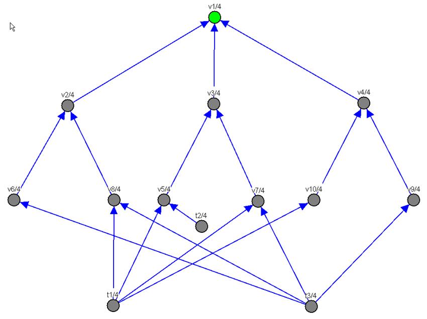
The shape of the database depends on
the randomizer, but the same result can be obtained with the same random seed.
To this end, you can use the flag random_seed as used above to
reproduce the same results as depicted.
There are other parameters that can
be set by setting system flags as follows:
· gen_number_of_table_columns(Number). % Number of columns in
both tables and views. Default: 4. Minimum: 2
· gen_column_type(InternalType). % Type of the columns. Default: number(integer).
Possible other values: number(float), string(varchar), string(varchar(N)), string(char(N)), where N is the
number of characters
· gen_children_density(Percent). % Probability (0-100) of having MaxChildren in each
node. Default: 70
Any of these flags can be modified
with the command: /set_flag FlagName
Value. For example, the following will set
the number of columns to 2:
/set_flag gen_number_of_table_columns 2
5.22 Notes about the Implementation of DES
DES is implemented with the original
ideas found in [Diet87, TS86, FD92], that deal with termination issues of
Prolog programs. These ideas have been already used in the deductive database
community. Our implementation uses extension tables for achieving a top–down
driven bottom–up approach. In its current form, it can be seen as an extension
of the work in [Diet87, FD92] in the sense that, in addition, we deal with
negation, undefined (although incomplete) information, nulls, aggregates, Top-N
queries, hypothetical reasoning, restricted predicates and more. Also, the
implementation follows a different approach: Instead of compiling rules, they
are interpreted.
DES does not pretend to be an
efficient system but a system capable of showing the nice aspects of the more
powerful form of logic we can find in Datalog systems w.r.t. relational
database systems.
5.22.1 Tabling[20]
DES uses an extension table which
stores answers to goals previously computed, as well as their calls. For the
ease of the introduction, we assume an answer table and a call table to store
answers and calls, respectively. Answers may be positive or negative, that is,
if a call to a positive goal p succeeds, then the fact p is added as an answer to the answer table; if a negated goal not p succeeds, then the fact not p is added. Calls are also added to the call table whenever they are
solved. This allows us to detect whether a call has been previously solved and
we can use the results in the extension table (if any).
The algorithm which implements this
idea is schematized next:
% Already called. Call table with an entry for the current call
memo(G) :-
build(G,Q), % Build in Q the same call with fresh variables
called(Q), % Look for a unifiable call in CT for the current call
subsumes(Q,G), % Test whether CT call subsumes
the current call
!, %
et_lookup(G). % If so, use the results in answer table (ET)
% New call. Call table without an entry for the current call
memo(G) :-
assertz(called(G)), % Assert the current call to CT
(
(et_lookup(G)) % First call returns all previous answers in ET
;
(solve_goal(G), % Solve the current call using applicable rules
build(G,Q), % Build in Q the same call with fresh variables
no_subsumed_by_et(Q), % Test whether there is no
entry in ET for Q
et_assert(G), % If so, assert the current result in ET
et_changed)). % Flag the change
This algorithm, first, tests whether
there is a previous call that subsumes[21] the current call. There are two possibilities: 1) there is such a
previous call: then, use the result in the answer table, if any. It is possible
that there is no such a result (for instance, when computing the goal p in the program p :- p) and we cannot derive any information, 2) otherwise, process the new
call knowing that there is no call or answer to this call in the extension
table. So, firstly store the current call and then, solve the goal with the
program rules (recursively applying this algorithm). Once the goal has been
solved (if succeeded), store the computed answer if there is no any previous
answer subsuming the current one (note that, through recursion, we can deliver
new answers for the same call). This so–called memoization process is
implemented with the predicate memo/1 in the file des.pl of the distribution, and will also be referred to as a memo function in
the rest of this manual.
Negative facts are produced when a
negative goal is proven by means of negation as failure (closed world
assumption). In this situation, a goal as not p which succeeds produces the fact not p which is added to the answer table, just the same as proving a positive
goal.
The command /list_et shows the
current state of the extension table, both for answers and calls already
obtained by solving one or more queries (incidentally, recall that you can
focus on the contents of the extension table for a given predicate, cf. Section
5.17.5). This command is useful for the
user when asking for the meaning of relations, and for the developer for
examining the last calls being performed. Before executing any query, the
extension table is empty; after executing a query, at least the call is not
empty. Also, the extension table is empty after the execution of a temporary
view.[22] The extension table contains the calls made during the last fixpoint
iteration (see next section for details); the calls are cleared before each
iteration whereas the answers are kept. The command /clear_et clears the
extension table contents, both for calls and answers.
5.22.2 Fixpoint Computation
The tabling mechanism is
insufficient in itself for computing all of the possible answers to a query.
The rationale behind this comes from the fact that the computed information is
not complete when solving a given goal, because it can use incomplete
information from the goals in its defining rules (these goals can be mutually
recursive). Therefore, we have to ensure that we produce all the possible
information by finding a fixpoint of the memo function. The algorithm
implementing this is depicted next:
solve_star(Q,St) :-
repeat,
(remove_calls, % Clear CT
et_not_changed, % Flag ET as not changed
solve(Q,St), % Solve the call to Q using memoization at stratum St
fail % Request all alternatives
;
no_change, % If no more alternatives, start a new iteration
!,
fail). % Otherwise, fail and
exit
First, the call table is emptied in
order to allow the system to try to obtain new answers for a given call,
preserving the previous computed answers. Then, the memo function is applied,
possibly providing new answers. If the answer table remains the same as before
after this last memo function application, we are done. Otherwise, the memo
function is reapplied as many times as needed until we find a stable answer
table (with no changes in the answer table). The answer table contains the meaning
of the query (plus perhaps other meanings for the relations used in the
computation of the given query).
The fixpoint is found in finite time
because the memo function is monotonic in the sense that we only add new
entries each time it is called while keeping the old ones. Repeatedly applying
the memo function to the answer table delivers a finite answer table since the
number of new facts that can be derived from a Datalog program is finite
(recall that there are no compound terms such as sk(z)). On the one hand, the number of positive facts which can be inferred
are finite because there is a finite number of ground facts which can be used
in a given proof, and proofs have finite depth provided that tabling prevents
recomputations of older nodes in the proof tree. On the other hand, the number
of negative facts which can be inferred is also finite because they are proved
using negation as failure. (Failures are always finite because they are proved
trying to get a success.) Finally, there are facts that cannot be proved to be
true or false because of recursion. These cases are detected by the tabling
mechanism which prevent infinite recursion such as in p :- p.
It is also possible that both a
positive and a negative fact have been inferred for a given call. Then, an
undefined fact replaces the contradictory information. The implementation
simply removes the contradictory facts and informs about the undefinedness. As
already indicated (see Section 6.8.1), the algorithm for determining
undefinedness is incomplete.
5.22.3 Dependency Graphs and Stratification: Negation, Outer Joins, and Aggregates
Each time a program is consulted or modified (i.e., via submitting a
temporary view or changing the database), a predicate dependency graph is built
[ZCF+97]. This graph shows the dependencies, through positive and negative atoms,
among predicates in the program. Also, a negative dependency is added for each
outer join goal and aggregate goal.
This dependency graph is useful for finding a stratification for the
program [ZCF+97]. A stratification collects predicates into numbered strata
(1..N). A basic bottom-up computation would solve all of the predicates in
stratum 1, then 2, and so on, until the meaning of the whole program is found.
With our approach, we only resort to compute by stratum when a negative
dependency occurs in the predicate dependency graph restricted to the query;
nevertheless, each predicate that is actually needed is solved by means of the
extension table mechanism described in the previous section. As a consequence,
many computations are avoided w.r.t. a naïve bottom-up implementation. See also
next section on optimizations.
Outer join and aggregate goals are also collected into strata as if they
were negative atoms in order to have their answer set completely defined and therefore
ensure termination of the computation algorithm in presence of null values (for
outer joins) and incomplete set of values (for aggregates).
5.22.4 Optimizations
Though, as already said, DES is not targeted at performance, it uses the
(slower in most systems) Prolog dynamic database, it does not allow
user-defined indexes, implemented algorithms are not the best ones, several
tasks are redone sparingly (although they can be actually saved), and so on.
Once that said, there has been still a minor room for optimizing performance so
that projects of the size DES is intended for can be successfully achieved.
Below, we list some of such optimizations that can be enabled or disabled at
user request (this feature is more oriented to the system implementors for
knowing the impact on performance of such optimizations). Each optimization is
listed in a subsection along with the command (between brackets) that is used
for disabling or enabling it (with the switch off and on, respectively).
5.22.4.1 Complete Computations (/optimize_cc)
Each call during the computation of a stratum (stratum saturation) is
remembered in addition to its outcome (in the answer table). Even when the
calls are removed in each fixpoint iteration (recall Section 5.22.2), most general ones do persist as a collateral
data structure to be used for saving computations should any of them is called
again during either computing a higher stratum or a subsequent query solving. 'cc' stands for completed computation,
so that if a call is marked as a completed computation, it is not even tried if
called again. This means the following two points: 1) During the computation of
the memo function, calls already computed are not tried to be solved again, and
only the entries in the memo table are returned. 2) Moreover, computing the
memo function is completely avoided if a subsuming already-computed call can be
found. In the first case, that saves solving goals in computing the memo
function. In the second case, that completely saves fixpoint computation.
The following system session shows how this optimization works. First,
we enable statistics collection, enable verbose output to automatically display
statistics results, disable all the optimizations, assert the fact p(1) and submit the query p(X):
DES> /statistics on
DES> /verbose on
DES> /optimize_cc
off
Info: Complete computations optimization is off.
DES> /optimize_ep
off
Info: Extensional predicate optimization is off.
DES> /optimize_nrp off
Info: Non-recursive predicates optimization is off.
DES> /optimize_st
off
Info: Stratum optimization is already disabled.
DES> /assert p(1)
Info: Rule asserted.
DES> p(X)
Info: Parsing query...
Info: DL query successfully parsed.
Info: Solving query p(X)...
Info: Displaying query answer...
Info: Sorting answer...
{
p(1)
}
Info: 1 tuple computed.
Info: Fixpoint iterations: 2
Info: EDB retrievals
: 2
Info: IDB retrievals
: 0
Info: ET retrievals
: 4
Info: ET look-ups : 6
Info: CT look-ups : 2
Info: CF look-ups : 0
Info: ET entries : 1
Info: CT entries : 1
As the statistics show, 2 fixpoint iterations have been needed to deduce
the output. In the first one, the rule p(1) is read for the first time. Then,
in the second iteration, it is read again and as the answer table has not
changed, then this means that the fixpoint has been reached. The information
display EDB retrievals shows those two fact reads (where EDB
stands for Extensional Database).
If the same query is submitted again:
DES> p(X)
Info: Parsing query...
Info: DL query successfully parsed.
Info: Solving query p(X)...
Info: Displaying query answer...
Info: Sorting answer...
{
p(1)
}
Info: 1 tuple computed.
Info: Fixpoint iterations: 1
Info: EDB retrievals
: 1
Info: IDB retrievals
: 0
Info: ET retrievals
: 4
Info: ET look-ups : 4
Info: CT look-ups : 1
Info: CF look-ups : 0
Info: ET entries : 1
Info: CT entries : 1
then only 1 iteration is needed to reach the fixpoint, and only one EDB
retrieval is done, as the answer table contained an entry for p(1) already for the same call. This
illustrates point 1 above.
Now let's enable the
optimization, previously deleting the contents of the answer table so that we
are in the same starting situation again:
DES> /clear_et
Info: Extension table cleared.
DES> /optimize_cc on
Info: Complete flag optimization is on.
DES> p(X)
Info: Parsing query...
Info: DL query successfully parsed.
Info: Solving query p(X)...
Info: Displaying query answer...
Info: Sorting answer...
{
p(1)
}
Info: 1 tuple computed.
Info: Fixpoint iterations: 2
Info: EDB retrievals
: 2
Info: IDB retrievals
: 0
Info: ET retrievals
: 4
Info: ET look-ups : 6
Info: CT look-ups : 2
Info: CF look-ups : 1
Info: ET entries : 1
Info: CT entries : 1
As before, 2 fixpoint
iterations and 2 EDB retrievals are needed. But, if we submit again the query:
DES> p(X)
Info: Parsing query...
Info: DL query successfully parsed.
Info: Solving query p(X)...
Info: Displaying query answer...
Info: Sorting answer...
{
p(1)
}
Info: 1 tuple computed.
Info: Fixpoint iterations: 0
Info: EDB retrievals
: 0
Info: IDB retrievals
: 0
Info: ET retrievals
: 2
Info: ET look-ups : 2
Info: CT look-ups : 0
Info: CF look-ups : 1
Info: ET entries : 1
Info: CT entries : 1
then, as the computation for the goal p(X) is complete, then no fixpoint
iterations are needed. For the same reason, no EDB retrievals are needed, as just
the contents of the memo table are returned. This illustrates point 2 above.
5.22.4.2 Extensional Predicates (/optimize_ep)
Extensional predicates are not needed to be iteratively computed. So, no
fixpoint computation is needed for them. They are known from the predicate
dependency graph simply because they occur in the graph without incoming arcs.
For them, a linear fetching is enough to derive their meanings. 'ep' stands for 'extensional
predicates'.
In the following system session we illustrate this with the fact p(1):
DES> /clear_et
Info: Extension table cleared.
DES> /optimize_ep on
Info: Extensional predicate optimization is on.
DES> p(X)
Info: Parsing query...
Info: DL query successfully parsed.
Info: Solving query p(X)...
Info: Displaying query answer...
Info: Sorting answer...
{
p(1)
}
Info: 1 tuple computed.
Info: Fixpoint iterations: 1
Info: EDB retrievals
: 1
Info: IDB retrievals
: 0
Info: ET retrievals
: 2
Info: ET look-ups : 3
Info: CT look-ups : 0
Info: CF look-ups : 1
Info: ET entries : 1
Info: CT entries : 1
where there are 1 fixpoint iteration and only one EDB retrieval. This
optimization is independent from the completed computations optimization.
Successive calls will render the same behaviour as in the previous
section, unless the complete computations optimization is enabled:
DES> p(X)
Info: Parsing query...
Info: DL query successfully parsed.
Info: Solving query p(X)...
Info: Displaying query answer...
Info: Sorting answer...
{
p(1)
}
Info: 1 tuple computed.
Info: Fixpoint iterations: 0
Info: EDB retrievals
: 0
Info: IDB retrievals
: 0
Info: ET retrievals
: 2
Info: ET look-ups : 2
Info: CT look-ups : 0
Info: CF look-ups : 1
Info: ET entries : 1
Info: CT entries : 1
where no fixpoint iterations and no EDB retrievals are needed.
5.22.4.3 Non-recursive Predicates (/optimize_nrp)
Each non-recursive predicate can be extracted out from the fixpoint
iterative cycle because its meaning can be computed by requesting all its
solutions at once. Further fixpoint iterations won't develop new tuples, so
this would be useless. In fact, this is true for each non-recursive rule of any
predicate (being recursive or not). Though, this optimization is not available
yet.
The following example shows the predicate p as composed of a fact and a rule.
First, it is computed with all optimizations disabled:
DES> /assert p(1)
DES> /assert p(X):-X=1+1
DES> p(X)
Info: Parsing query...
Info: DL query successfully parsed.
Info: Solving query p(X)...
Info: Displaying query answer...
Info: Sorting answer...
{
p(1),
p(2)
}
Info: 2 tuples computed.
Info: Fixpoint iterations: 2
Info: EDB retrievals
: 2
Info: IDB retrievals
: 2
Info: ET retrievals
: 8
Info: ET look-ups : 8
Info: CT look-ups : 2
Info: CF look-ups : 0
Info: ET entries : 2
Info: CT entries : 1
Then, enabling non-recursive predicates optimization and submitting the
same query:
DES> /optimize_nrp on
Info: Non-recursive predicates optimization is on.
DES> /clear_et
DES> p(X)
{
p(1),
p(2)
}
Info: 2 tuples computed.
Info: Fixpoint iterations: 1
Info: EDB retrievals
: 1
Info: IDB retrievals
: 1
Info: ET retrievals
: 4
Info: ET look-ups : 4
Info: CT look-ups : 0
Info: CF look-ups : 0
Info: ET entries : 2
Info: CT entries : 0
In only one fixpoint iteration the meaning is computed for which 1 EDB
and 1 IDB retrievals are needed (the fact and rule, respectively).
5.22.4.4 Stratum (/optimize_st)
Predicates which contain no recursive rules but calls to recursive
predicates do not need to be computed in the same iterative fixpoint
computation. If this optimization is enabled, such predicates are isolated from
recursive ones in another stratum, so that iterative cycles are saved for them.
This situation occurs, for instance, when compiling SQL queries to Datalog, as
the intermediate relation answer is introduced. Next system session
illustrates this:
DES> :-type(p(a:int))
DES> /display_answer off
DES> /display_nbr_of_tuples off
DES> /timing on
DES> /running_info off
DES> /assert p(1)
DES> /assert p(X):-p(Y),X=Y+1,Y<500
DES> select * from p
Info: Solving query answer(A)...
answer(p.a:int) ->
Info: Fixpoint iterations: 500
Info: EDB retrievals
: 500
Info: IDB retrievals
: 1000
Info: ET retrievals
: 627246
Info: ET look-ups : 252999
Info: CT look-ups : 1500
Info: CF look-ups : 0
Info: ET entries : 1000
Info: CT entries : 2
Info: Total elapsed time: 02.755 s.
DES> /optimize_st
on
DES> select * from p
Info: Solving query answer(A)...
Info: Computing by stratum of [p(A)].
answer(p.a:int) ->
Info: Fixpoint iterations: 2
Info: EDB retrievals
: 502
Info: IDB retrievals
: 504
Info: ET retrievals
: 381248
Info: ET look-ups : 128757
Info: CT look-ups : 1006
Info: CF look-ups : 0
Info: ET entries : 1000
Info: CT entries : 2
Info: Total elapsed time: 01.888 s.
With this optimization enabled, less extension table lookups are needed
and the result is therefore computed faster. However, note that non-termination
might raise when breaking strata if using the metapredicate top: This is because top requires the amount of tuples as
indicated from its goal argument. If this goal is isolated in a higher stratum,
no top constraint is propagated to the lower stratum, as in:
DES> :- type(p(a:int))
DES> /assert p(1)
DES> /assert p(X):-p(Y),X=Y+1
DES> select top 2 * from p
answer(p.a:int) ->
{
answer(1),
answer(2)
}
Info: 2 tuples computed.
DES> /optimize_st on
DES> select top 2 * from p
... non-terminating query
That is, as the SQL query had been compiled to:
answer(A) :-
top(10,p(A)).
then, the predicate answer/1 is located at stratum 2 and the
predicate p/1 at stratum 1:
DES> /strata
[(p/1,1),(answer/1,2)]
and DES tries to solve first the goal p(X) (not top(10,p(A)))[23] which proves to be non-terminating
as there is no top constraint on p. Further releases might cope with
this issue.
5.22.5 Indexing (/indexing)
There is no provision for user indexes up to now. However, indexing on
memo tables can be enabled or disabled at user request. There are three tables
which are indexed: the answer table, the call table, and the complete
computation table. The first one stores the computed results for the calls
during query solving and it is used in the tabling scheme for avoiding to
recompute already known goals. The second one stores the calls so that it is
possible to know whether a subsuming call has been done already. The third
table stores for each call whether its computation has been either completed or
not.
The next system session shows a speed-up of almost 3×
when enabling indexing.
DES> /timing on
DES> /indexing off
DES> /pretty_print off
DES> /display_answer off
DES> p(X):-X=1;p(Y),Y<500,X=Y+1
Info: Processing:
p(X)
in the program context of the exploded
query:
p(X) :- X=1.
p(X) :- p(Y),Y<500,X=Y+1.
Info: 500 tuples computed.
Info: Total elapsed time: 03.540 s.
DES> /indexing on
DES> p(X):-X=1;p(Y),Y<500,X=Y+1
Info: Processing:
p(X)
in the program context of the exploded
query:
p(X) :- X=1.
p(X) :- p(Y),Y<500,X=Y+1.
Info: 500 tuples computed.
Info: Total elapsed time: 01.279 s.
5.22.6 Porting to Unsupported Systems
DES is implemented in several Prolog
files:
· des.pl contains the common predicates for all of the platforms (both Prolog
interpreters and operating systems) following the Prolog ISO standard.
· des_ini.pl contains initialization directives for loading files at system start-up.
· des_dcg.pl contains the definition of DCG expansion (which varies from one Prolog system
to another).
·
des_sql.pl contains the SQL processor.
· des_ra.pl contains the RA processor.
· des_drc.pl contains the DRC processor.
· des_trc.pl contains the TRC processor.
· des_commands.pl defines system commands.
· des_help.pl includes the help system.
· des_common.pl includes predicates used by several files.
· des_types.pl contains the type checking, inference and casting systems.
· des_atts.pl for allowing attributed variables in the context of types.
· des_modes.pl implements the mode information system for Datalog predicates.
· des_persistence.pl implements persistence of Datalog predicates on external SQL databases
via ODBC connections.
· des_fuzzy.pl implements a fuzzy system.
· des_trace.pl implements a naïve declarative tracer.
· des_dl_debug.pl contains the Datalog declarative debugger.
·
des_sql_debug.pl contains the SQL declarative debugger.
·
des_sql_semantic.pl contains the SQL semantic checker.
· debug/des_pchr.pl is a CHR program for debugging Datalog predicates
and used by des_dl_debug.pl.
· des_tc.pl contains the SQL test case generator code.
· des_dbigen.pl contains the SQL database instance random generator.
· des_glue.pl contains Prolog system specific code, which vary from a system to
another.
Adapting the predicates found in the
last file should not pose problems, provided that the Prolog interpreter and
operating system feature some required characteristics. In particular, finite
domain constraints with positive and negative integers is a must for supporting
several features of DES, such as type inference and test case generation. Also,
attributed variables are required. Finally, file-system-related built-ins. If
you plan to port DES to other systems not described here, you will have to
modify the system specific Prolog file to suit your system. If so, and if you
want to figure as one of the system contributors, please send an e–mail message
with the code and reference information to: fernan@sip.ucm.es, accepting that your contribution will be under the GNU Lesser General
Public License. (See the appendix for details.)
6. Examples
The DES distribution contains the directory examples, with many program examples and scripts. Next, a few of them are
explained. Unless explicitly noted, all queries have been solved after the
commands /verbose off and /pretty_print off have been executed.
6.1 Relational Operations (files relop.{dl,sql,ra,drc,trc})
The program
relop.dl is intended to show how to mimic
with Datalog rules the basic relational operations that can be found in the
file relop.sql. It contains three relations (a, b, and c), which
are used as arguments of relational operations. In order to have loaded this
program and be able to submit queries you can consult it with /c relop.
In the remarks below, relational operator symbols are represented with ASCII
characters, as =|x| to denote the left outer join ![]()
![]() , the letter x to simply denote the Cartesian product, and the letter U for the set union.
, the letter x to simply denote the Cartesian product, and the letter U for the set union.
% (Extended) Relational Algebra Operations
% pi(X)(c(X,Y)) : Projection of the first argument of c
projection(X)
:- c(X,Y).
% sigma(X=a2)(a) : Selecting tuples from a such that its first argument
is a2
selection(X)
:- a(X), X=a2.
% a x b : Cartesian product of relations a and b
cartesian(X,Y) :- a(X), b(Y).
% a |x| b : Natural inner join of relations a and b
inner_join(X) :- a(X), b(X).
% a =|x| b : Left outer join of relations a and b
left_join(X,Y) :- lj(a(X), b(Y), X=Y).
% a |x|= b : Right outer join of relations a and b
right_join(X,Y) :- rj(a(X), b(Y), X=Y).
% a =|x|= b : Full outer join of relations a and b
full_join(X,Y) :- fj(a(X), b(Y), X=Y).
% a U b : Set union of relations a and b
union(X) :- a(X) ; b(X).
% a - b: Set difference of relations a and b
difference(X) :- a(X), not b(X).
Once the
program is consulted, you can query it with, for example:
DES> projection(X)
{
projection(a1),
projection(a2)
}
Info: 2 tuples computed.
The result
of a query is the meaning of the view, i.e., the fact set for the query derived
from the program whether intensionally or extensionally. In the above example, projection(X) corresponds to the projection of
the first argument of relation c.
The second
view in Section 4.1.5 returns:
Info: Processing:
a(X) :- b(X).
{
a(a1),
a(a2),
a(a3),
a(b1),
a(b2)
}
Info: 5 tuples computed.
For
abolishing this program and execute the SQL statements in relop.sql, you can type /abolish and /process relop.sql.
Note that the extension can be omitted in the /process command.
Here, we
depart from the Datalog interpreter and, if you are to submit SQL queries, it
is useful to switch to the SQL interpreter via the command /sql as inputs will be parsed only by the SQL
parser. Otherwise, it will be tried to be identified as a Datalog input, and
then as an SQL input.
Note that in
the file relop.sql listed below, strings are enclosed
between apostrophes. This is not needed in the Datalog language. In order to
execute the contents of this file, type /process relop.sql.
% Switch to SQL interpreter
/sql
% Creating tables
create or replace table a(a);
create or replace table b(b);
create or replace table c(a,b);
% Listing the database schema
/dbschema
% Inserting values into tables
insert into a values ('a1');
insert into a values ('a2');
insert into a values ('a3');
insert into b values ('b1');
insert into b values ('b2');
insert into b values ('a1');
insert into c values ('a1','b2');
insert into c values ('a1','a1');
insert into c values ('a2','b2');
% Testing the just inserted values
select * from a;
select * from b;
select * from c;
% Projection
select a from c;
% Selection
select a from a where a='a2';
% Cartesian product
select * from a,b;
% Inner Join
select a from a inner join b on a.a=b.b;
% Left Join
select * from a left join b on a.a=b.b;
% Right Join
select * from a right join b on a.a=b.b;
% Full Join
select * from a full join b on a.a=b.b;
% Union
select * from a union select * from b;
% Difference
select * from a except select * from b;
If we have
created the relations in Datalog, we cannot access them from SQL unless they
had been either defined as tables or views or declared with types. For example,
following the first alternative and after consulting the file relop.dl, we can submit:
create table a(a varchar);
And, then,
accessing with an SQL statement the tuples that were asserted in Datalog:
DES> select * from a;
answer(a.a) ->
{
answer(a1),
answer(a2),
answer(a3)
}
Info: 3 tuples computed.
Otherwise,
an error is submitted:
Error:
Unknown table or view 'a'.
Following
the second alternative, and after consulting the file relop.dl, we can declare types for a:
DES> /datalog :-type(a,[a:varchar])
DES> select * from a
answer(a.a) ->
{
answer(a1),
answer(a2),
answer(a3)
}
Info: 3 tuples computed.
Files relop.trc and relop.drc
include the relational operations expressed as queries in these files. To
process any of these files you have to proceed similar to SQL: /p relop.trc, for instance. As an example or TRC, the
following computes the set union of two relations:
DES-TRC>
{X|a(X) or b(X)};
answer(a:string) ->
{
answer(a1),
answer(a2),
answer(a3),
answer(b1),
answer(b2)
}
Info: 5 tuples computed.
6.2 Paths in a Graph (files paths.{dl,sql,ra})
This
program[24] introduces the use of recursion in
DES by defining the graph in Figure 2 and the set of tuples <origin,
destination> such that there is a path from origin to destination.
Figure 2. Paths in a Graph
The file paths.dl contains the following Datalog code, which can
be consulted with /c paths:
% Paths in a Graph
edge(a,b).
edge(a,c).
edge(b,a).
edge(b,d).
path(X,Y) :- path(X,Z), edge(Z,Y).
path(X,Y) :- edge(X,Y).
The query path(X,Y) yields the following answer:
{
path(a,a),
path(a,b),
path(a,c),
path(a,d),
path(b,a),
path(b,b),
path(b,c),
path(b,d)
}
Info: 8 tuples computed.
The file paths.sql contains the SQL counterpart code, which can
be executed with /process
paths.sql:
create table edge(origin,destination);
insert into edge values('a','b');
insert into edge values('a','c');
insert into edge values('b','a');
insert into edge values('b','d');
create view paths(origin,destination) as
with
recursive path(origin,destination) as
(select * from edge)
union
(select path.origin,edge.destination
from path,edge
where path.destination = edge.origin)
select * from path;
So, you can
get the same answer as before with the SQL statement:
DES> select * from paths;
answer(paths.origin, paths.destination) ->
{
answer(a,a),
answer(a,b),
answer(a,c),
answer(a,d),
answer(b,a),
answer(b,b),
answer(b,c),
answer(b,d)
}
Info: 8 tuples computed.
Another
shorter formulation is allowed in DES with the following view definition:
create view path(origin,destination) as
select * from
(select * from edge)
union
(select path.origin,edge.destination
from path,edge
where path.destination=edge.origin)
You can
finally compare this with the RA formulation:
paths(origin,destination) :=
select true (edge)
union
project paths.origin,edge.destination
(edge zjoin paths.destination = edge.origin paths);
6.3 Shortest Paths (file spaths.{dl,sql,ra})
Thanks to
aggregate predicates, one can code the following version of the shortest paths
problem (file spaths.dl), which uses the same definition of
edge as in the previous example:
path(X,Y,1) :-
edge(X,Y).
path(X,Y,L) :-
path(X,Z,L0),
edge(Z,Y),
count(edge(A,B),Max),
L0<Max,
L is L0+1.
sp(X,Y,L) :-
min(path(X,Y,Z),Z,L).
Note that
the infinite computation that may raise from using the built-in is/2 is avoided by limiting the total length of a
path to the number of edges in the graph.
The
following query returns all the possible paths and their corresponding minimal
distances:
DES> sp(X,Y,L)
{
sp(a,a,2),
sp(a,b,1),
sp(a,c,1),
sp(a,d,2),
sp(b,a,1),
sp(b,b,2),
sp(b,c,2),
sp(b,d,1)
}
Info: 8 tuples computed.
Below is
the SQL formulation for the same problem (file spaths.sql)
:
DES> create or replace view spaths(origin,destination,length) as with recursive path(origin,destination,length) as
(select edge.*,1 from edge)
union
(select path.origin,edge.destination,path.length+1
from path,edge
where path.destination=edge.origin and
path.length<(select count(*) from edge))
select origin,destination,min(length) from path group by origin,destination;
DES> select * from spaths
answer(spaths.origin, spaths.destination, spaths.length) ->
{
answer(a,a,2),
answer(a,b,1),
answer(a,c,1),
answer(a,d,2),
answer(b,a,1),
answer(b,b,2),
answer(b,c,2),
answer(b,d,1)
}
Info: 8 tuples computed.
A possible
RA formulation follows:
max_length(max_length) :=
group_by [] count(*) true (edge);
path(origin,destination,length) :=
project origin,destination,1 (edge)
union
project path.origin,edge.destination,path.length+1
(
path
zjoin path.destination=edge.origin and
path.length<max_length
(edge product max_length)
);
spaths(origin,destination,length) :=
group_by origin,destination origin,destination,min(length) true
(path);
And its
query:
/ra select true (spaths);
6.4 Family Tree (files family.{dl,sql,ra})
This (yet
another classic) program defines the family tree shown in Figure 3, the set of tuples <parent,child> such that parent is a parent of child (the relation parent), the set of tuples <ancestor,descendant> such that ancestor is an ancestor of descendant (the relation ancestor), the set of tuples <father,child> such that father is the father of child (the relation father), and the set of tuples <mother,child> such that mother is the mother of child (the relation mother).
Figure 3. Family Tree
The file family.dl contains the following Datalog code, which can
be consulted with /c family:
father(tom,amy).
father(jack,fred).
father(tony,carolII).
father(fred,carolIII).
mother(grace,amy).
mother(amy,fred).
mother(carolI,carolII).
mother(carolII,carolIII).
parent(X,Y) :- father(X,Y).
parent(X,Y) :- mother(X,Y).
ancestor(X,Y) :- parent(X,Y).
ancestor(X,Y) :- parent(X,Z), ancestor(Z,Y).
The query ancestor(tom,X) yields the following answer (that is, it
computes the set of descendants of tom):
{
ancestor(tom,amy),
ancestor(tom,carolIII),
ancestor(tom,fred)
}
Info: 3 tuples computed.
Solving the
view:
son(S,F,M) :- father(F,S),mother(M,S).
yields the following answer, computing the set of sons:
Info: Processing:
son(S,F,M) :- father(F,S),mother(M,S).
{
son(amy,tom,grace),
son(carolII,tony,carolI),
son(carolIII,fred,carolII),
son(fred,jack,amy)
}
Info: 4 tuples computed.
The file family.sql contains the SQL counterpart code, which can
be executed with /process
family.sql:
create table father(father,child);
insert into father values('tom','amy');
insert into father values('jack','fred');
insert into father values('tony','carolII');
insert into father values('fred','carolIII');
create table mother(mother,child);
insert into mother values('grace','amy');
insert into mother values('amy','fred');
insert into mother values('carolI','carolII');
insert into mother values('carolII','carolIII');
create view parent(parent,child) as
select * from father
union
select * from mother;
create or replace view ancestor(ancestor,descendant) as
select parent,child from parent
union
select parent,descendant from parent,ancestor
where parent.child=ancestor.ancestor;
The two
example queries above can be formulated in SQL as:
select * from ancestor where ancestor='tom';
select child,father,mother
from father,mother
where father.child=mother.child;
And also as
RA queries as:
/ra select ancestor='tom' (ancestor);
project child,father,mother
(father zjoin father.child=mother.child mother);
6.5 Basic Recursion Problem (file recursion.dl)
This
example is intended to show that queries involving recursive predicates do
terminate thanks to DES fixpoint solving, by contrast with Prolog’s usual SLD
resolution.
p(0).
p(X)
:- p(X).
p(1).
The query p(X) returns the inferred facts from the
program irrespective of the apparent infinite recursion in the second rule.
(Note that the Prolog goal p(1) does not terminate. You can easily check it
out with /prolog
p(1).)
6.6 Transitive Closure (files tranclosure.{dl,sql,ra})
With this
example, we show a possible use of mutual recursion by means of a Datalog program
that defines the transitive closure of the relations p and q[25]. It can be consulted with /c tranclosure.
p(a,b).
p(c,d).
q(b,c).
q(d,e).
pqs(X,Y) :- p(X,Y).
pqs(X,Y) :- q(X,Y).
pqs(X,Y) :- pqs(X,Z),p(Z,Y).
pqs(X,Y) :- pqs(X,Z),q(Z,Y).
The query pqs(X,Y) returns the whole set of inferred facts that
model the transitive closure.
File tranclosure.sql contains the SQL counterpart code, which can
be executed with /process
tranclosure.sql:
create table p(x,y);
insert into p values ('a','b');
insert into p values ('c','d');
create table q(x,y);
insert into q values ('b','c');
insert into q values ('d','e');
create view pqs(x,y) as
select * from p
union
select * from q
union select pqs.x,p.y from pqs,p where pqs.y=p.x
union select pqs.x,q.y from pqs,q where pqs.y=q.x;
The query select * from pqs returns the same answer as before.
The file tranclosure.ra contains the RA formulation:
pqs(x,y) :=
p
union
q
union
project pqs.x,p.y (pqs zjoin pqs.y=p.x p)
union
project pqs.x,q.y (pqs zjoin pqs.y=q.x q);
/ra select true (pqs)
6.7
Mutual
Recursion (files mutrecursion.{dl,sql,ra})
The
following program shows a basic example about mutual recursion:
p(a).
p(b).
q(c).
q(d).
p(X)
:- q(X).
q(X)
:- p(X).
Submitting
the goal p(X), we get:
{
p(a),
p(b),
p(c),
p(d)
}
Info: 4 tuples computed.
which is the same set of values for arguments for the query q(X). The file mrtc.dl is a combination of this example and that of
the previous section.
The file mutrecursion.sql contains the SQL counterpart code, which can
be executed with /process
mutrecursion.sql:
/sql
/assert p(a)
/assert p(b)
/assert q(c)
/assert q(d)
-- View q must be given a prototype for view p to be defined
create view q(x) as select * from q;
create or replace view p(x) as select * from q;
create or replace view q(x) as select * from p;
Note that
it is needed to build a void view for q in order to have it declared when
defining the view p. The void view is then replaced by its actual
definition. The contents of both views can be tested to be equal with:
select * from p;
select * from q;
File mutrecursion.ra contains the RA formulation:
-- View q must be given a prototype for view p to be defined
q(x)
:= select true (q);
p(x)
:= select true (q);
q(x)
:= select true (p);
select true (p);
select true (q);
6.8 Farmer-Wolf-Goat-Cabbage Puzzle (file puzzle.dl)
This
example[26] shows the classic
Farmer–Wolf–Goat–Cabbage puzzle (also Missionaries and Cannibals as another
rewritten form). The farmer, wolf, goat, and cabbage are all on the north shore
of a river and the problem is to transfer them to the south shore. The farmer
has a boat which he can row taking at most one passenger at a time. The goat
cannot be left with the wolf unless the farmer is present. The cabbage, which counts
as a passenger, cannot be left with the goat unless the farmer is present. The
following program models the solution to this puzzle. The relation state/4 defines the valid states under
the specification (i.e., those situations in which there is no danger for any
of the characters in our story; a state in which the goat is left alone with
the cabbage may result in an eaten cabbage) and imposes that there is a
previous valid state from which we depart from. The arguments of this relation
are intended to represent (from left to right) the position (north –n– or south –s– shore) of the farmer, wolf, goat,
and cabbage. We use the relation safe/4 to verify that a given configuration of
positions is valid. The relation opp/2 simply states that north is the opposite
shore of south and vice versa.
% Initial state
state(n,n,n,n).
% Farmer takes Wolf
state(X,X,U,V) :-
safe(X,X,U,V),
opp(X,X1),
state(X1,X1,U,V).
% Farmer takes Goat
state(X,Y,X,V) :-
safe(X,Y,X,V),
opp(X,X1),
state(X1,Y,X1,V).
% Farmer takes Cabbage
state(X,Y,U,X) :-
safe(X,Y,U,X),
opp(X,X1),
state(X1,Y,U,X1).
% Farmer goes by himself
state(X,Y,U,V) :-
safe(X,Y,U,V),
opp(X,X1),
state(X1,Y,U,V).
% Opposite shores (n/s)
opp(n,s).
opp(s,n).
% Farmer is with Goat
safe(X,Y,X,V).
% Farmer is not with Goat
safe(X,X,X1,X) :- opp(X,X1).
If we
submit the query state(s,s,s,s), we get the expected result:
{
state(s,s,s,s)
}
Info: 1 tuple computed.
That is,
the system has proved that there is a serial of transfers between shores which finally
end with the asked configuration (this problem is not modelled to show this
serial). If we ask for the extension table contents regarding the relation state/4 (with the command /list_et state/4), we get for the answers:
{
state(n,n,n,n),
state(n,n,n,s),
state(n,n,s,n),
state(n,s,n,n),
state(n,s,n,s),
state(s,n,s,n),
state(s,n,s,s),
state(s,s,n,s),
state(s,s,s,n),
state(s,s,s,s)
}
Info: 10 tuples in the answer set.
This is the
complete set of valid states which includes all of the valid paths from state(n,n,n,n) to state(s,s,s,s). However, the order of states to
reach the latter is not given, but we can find it by observing this relation,
i.e.:
state(n,n,n,n) ® Farmer takes Goat to south shore ®
state(s,n,s,n) ® Farmer returns to north shore ®
state(n,n,s,n) ® Farmer takes Wolf to south shore ®
state(s,s,s,n) ® Farmer takes Goat to north shore ®
state(n,s,n,n) ® Farmer takes Cabbage to south shore ®
state(s,s,n,s) ® Farmer returns to north shore ®
state(n,s,n,s) ® Farmer takes Goat to south shore ®
state(s,s,s,s)
Final safe state
Observe
that there is two states in the relation state/4 which do not form part of the
previous path:
state(s,n,s,s)
state(n,n,n,s)
These
states come from another possible path:[27]
state(n,n,n,n) ® Farmer takes Goat to south shore ®
state(s,n,s,n) ® Farmer returns to north shore ®
state(n,n,s,n) ® Farmer takes Cabbage to south shore ®
state(s,n,s,s) ® Farmer takes Goat to north shore ®
state(n,n,n,s) ® Farmer takes Wolf to south shore ®
state(s,s,s,n) ® Farmer takes Goat to north shore ®
state(s,s,n,s) ® Farmer returns to north shore ®
state(n,s,n,s) ® Farmer takes Goat to south shore ®
state(s,s,s,s)
Final safe state
6.8.1 Dealing with paths (file puzzle1.dl)
As just illustrated, the sequence of movements
needed to find a feasible solution can be inferred from the answer table.
Nonetheless, it is possible to outcome such sequences even when there is no
provision for data structures. The idea is to code sequences of movements into
a single plain type, as an integer. We can resort, for instance, to build a
decimal number whose digits, as read from right
to left, indicate the selected movement in the sequence. If we number the
movement alternatives from 1 to 4 (in the same order as rules occur at the
program text) the first solution above can be coded as 2412342, and the second
one as 2432142.
Modelling in this way, we can rewrite the
predicate state by adding a first argument as the sequence needed to reach a
given state, and the steps already performed. This is useful to build the code
as adding a number (identifying the alternative rule) multiplied by the n-th power of ten, where n is the number of steps already done. The
following two example rules illustrates this:
% 0. Initial state
state(0,0,n,n,n,n).
% 1. Farmer takes Wolf
state(C,S,X,X,U,V) :-
safe(X,X,U,V),
opp(X,X1),
state(C1,S1,X1,X1,U,V),
S is S1+1,
bound(B),
S<B,
C is C1+1*10**S1.
Solving the new program yields:
DES> state(C,S,s,s,s,s)
{
state(2412342.0,7,s,s,s,s),
state(2432142.0,7,s,s,s,s)
}
Info: 2 tuples
computed.
Which is explained as follows:
* Solution 1: state(2412342.0,7,s,s,s,s)
0: Initial state
North: Farmer,Goat,Cabbage,Wolf
South: empty
2: Farmer takes goat to the South shore
North: Cabbage,Wolf
South: Farmer,Goat
4: Farmer returns to North shore
North: Farmer,Cabbage,Wolf
South: Goat
3: Farmer takes cabbage to the South shore
North: Wolf
South: Farmer,Cabbage,Goat
2: Farmer takes goat to the North shore
North:
Farmer,Goat,Wolf
South: Cabbage
1: Farmer takes wolf to the South shore
North: Goat
South: Farmer,Cabbage,Wolf
4: Farmer returns to North shore
North: Farmer,Goat
South: Cabbage,Wolf
2: Farmer takes goat to the South shore
North: empty
South: Farmer,Goat,Cabbage,Wolf
* Solution 2: state(2432142.0,7,s,s,s,s)
0: Initial state
North: Farmer,Goat,Cabbage,Wolf
South: empty
2: Farmer takes goat to the South shore
North: Cabbage,Wolf
South: Farmer,Goat
4: Farmer returns to North shore
North: Farmer,Cabbage,Wolf
South: Goat
1: Farmer takes wolf to the South shore
North: Cabbage
South: Farmer,Goat,Wolf
2: Farmer takes goat to the North shore
North: Farmer,Goat,Cabbage
South: Wolf
3: Farmer takes cabbage to the South shore
North: Goat
South: Farmer,Cabbage,Wolf
4: Farmer returns to North shore
North: Farmer,Goat
South: Cabbage,Wolf
2: Farmer takes goat to the South shore
North: empty
South: Farmer,Goat,Cabbage,Wolf
6.9 Paradoxes (files russell.{dl,sql,ra})
When
negation is used, we can find paradoxes, such as the Russell’s paradox (the
barber in a town shaves every person who does not shave himself) shown in the
next example (please note that this example is not stratified and, in general,
we cannot ensure correctness for non-stratifiable programs):
DES> /verbose on
Info: Verbose output is on.
DES> /c russell
Info: Consulting russell...
man(barber).
man(mayor).
shaves(barber,M) :-
man(M),
not shaves(M,M).
shaved(M) :-
shaves(barber,M).
end_of_file.
Info: 4 rules consulted.
Info: Computing predicate dependency graph...
Info: Computing strata...
Warning: Non stratifiable program.
If we
submit the query shaves(X,Y), we get the positive facts as well as a set of
undefined inferred information (in our example, whether the barber shaves
himself), as follows (here, verbose output is enabled):
DES> shaves(X,Y)
Warning: Unable to ensure correctness for this query.
{
shaves(barber,mayor)
}
Info: 1 tuple computed.
Undefined:
{
shaves(barber,barber)
}
Info: 1 tuple undefined.
If we look
at the extension table contents by submitting the command /list_et, we get as answers:
Answers:
{
man(barber),
man(mayor),
not shaves(mayor,mayor),
shaves(barber,mayor)
}
Info: 4 tuples in the answer set.
We can see
that, in particular, we have proved additional negative information (the mayor
does not shaves himself) and that no information is given for the undefined
facts. The current implementation uses an incomplete algorithm for finding such
undefined facts. We can see this incompleteness by adding the following rule:
shaved(M) :- shaves(barber,M).
The query shaved(M) returns:
Warning: Unable to
ensure correctness for this query.
{
shaved(mayor)
}
Info: 1 tuple computed.
That is,
the system is unable to prove that shaved(barber) is undefined.
If you look
at the predicate dependency graph and the stratification of the program:
DES> /pdg
Nodes:
[man/1,shaved/1,shaves/2]
Arcs
: [shaves/2-shaves/2,shaves/2+man/1,shaved/1+shaves/2]
DES> /strata
[non-stratifiable]
you get the predicate dependency graph shown in Figure 4, and you are informed that the
program is non-stratifiable. This figure shows a negation in a cycle, so that
the program is not stratifiable. (The system warned of this situation when the
program was loaded.)

Figure 4. Predicate Dependency Graph for russell.dl
However, even when a program is
non-stratifiable, there may exist a query with an associated predicate
dependency subgraph so that negation does not occur in any cycle. For instance,
this occurs with the query man(X) in this program:
DES> man(X)
Info: Stratifiable subprogram found for the given query.
{
man(barber),
man(mayor)
}
Info: 2 tuples computed.
Here, the
system recomputed the strata for the predicate dependency subgraph, and
informed that it found a stratifiable subprogram for such a query. In this
simple case, no more negations were involved in the subgraph, but more
elaborated dependencies can be found in other examples (cf. sections 6.10 and 6.11).
Stratification
may be needed for programs without negation as long as a temporary view
contains a negated goal. Consider the following view under the program relop.dl (rules in the program with negation are not
present in the subgraph for the query d(X)):
DES> d(X) :- a(X), not b(X)
Info: Processing:
d(X) :- a(X),not b(X).
{
d(a2),
d(a3)
}
Info: 2 tuples computed.
In this
view, the query d(X) is solved with a solve-by-stratum algorithm,
described in Section 5.22.3. In this case, this means that the
goal b(X) is solved before obtaining the meaning of d(X) because b is in a lower stratum than d and it is needed for the
computation of d.
The basic
paradox p:-not p can be
found in the file paradox.dl, whose model is undefined as you
can test with the query p.
6.10 Parity (file DLDebugger/parity.dl)
This example program[28] is intended to compute the parity of a given base relation br(X), i.e., it can determine whether the number of elements in the relation
(cardinality) is even or odd by means of the predicates br_is_even, and br_is_odd, respectively.
The predicate next defines an ascending chain of elements in br based on their textual ordering, where the first link of the chain
connects the distinguished node nil to the first element in br. The predicates even and odd define the even, resp. odd, elements in the chain. The predicate has_preceding defines the elements in br such that there are previous
elements to a given one (the first element in the chain has no preceding
elements). The rule defining this predicate includes an intended error (fourth
rule in the example) which will be used in Section 6.13 to show how it is caught by the declarative debugger.
% Pairs of
non-consecutive elements in br
between(X,Z) :-
br(X), br(Y), br(Z), X<Y, Y<Z.
% Consecutive elements
in the sequence, starting at nil
next(X,Y) :-
br(X), br(Y), X<Y, not between(X,Y).
next(nil,X) :-
br(X), not has_preceding(X).
% Values having
preceding values in the sequence
has_preceding(X) :-
br(X), br(Y), Y>X. % Error: Y>X should
be Y<X
% Values in an even
position of the sequence, including nil
even(nil).
even(Y) :-
odd(X), next(X,Y).
% Values in an odd
position of the sequence
odd(Y) :-
even(X), next(X,Y).
% Succeeds if the
cardinality of the sequence is even
br_is_even :-
even(X), not next(X,Y).
% Succeeds if the
cardinality of the sequence is odd
br_is_odd :-
odd(X), not next(X,Y).
% Base relation
br(a).
br(b).
6.11 Grammar (file grammar.dl)
Parsers can also be coded as Datalog programs. In this example[29], a simple left-recursive grammar
analyser is coded for the following grammar rules.
A –> a
A –> Ab
A –> Aa
It was tested with the input string "ababa", which is coded with the
relation t(F,T,L), F for the position of token T that ends at position L.
t(1,a,2).
t(2,b,3).
t(3,a,4).
t(4,b,5).
t(5,a,6).
a(F,L) :- t(F,a,L).
a(F,L) :- a(F,M), t(M,b,L).
a(F,L) :- a(F,M), t(M,a,L).
DES> a(1,6)
{
a(1,6)
}
Info: 1 tuple computed.
6.12
Fibonacci
(file fib.{dl,sql,ra})
The all-time classics Fibonacci program[30] can be coded in DES thanks to
arithmetic built-ins. It can be formulated as follows:
fib(0,1).
fib(1,1).
fib(N,F) :-
N>1,
N2 is N-2,
fib(N2,F2),
N1 is N-1,
fib(N1,F1),
F is F2+F1.
Since DES is implemented with extension tables, computing high Fibonacci
numbers is possible with linear complexity:
DES> fib(
{
fib(1000,70330367711422815821835254877183549770181269836358732742604905087154537118196933579742249494562611733487750449241765991088186363265450223647106012053374121273867339111198139373125598767690091902245245323403501)
}
Info: 1 tuple computed.
Also, it is possible to formulate this in SQL, even when the next view
features non-linear recursion (file fib.sql):
create view fib(n,f) as
select 0,1
union
select 1,1
union
select fib1.n+1,fib1.f+fib2.f
from fib fib1, fib fib2
where fib1.n=fib2.n+1 and fib1.n<10;
As well, next there is a possible RA formulation (file fib.ra):
fib(n,f) :=
project 0,1 (dual)
union
project 1,1 (dual)
union
project fib1.n+1,fib1.f+fib2.f
(rename fib1(n1,f1) (fib)
zjoin
n1=n2+1 and n1<10
rename fib2(n2,f2) (fib));
6.13 Hanoi Towers (file hanoi.dl)
Another well-known toy puzzle is the towers of
Hanoi, which can be coded as:
hanoi(1,A,B,C).
hanoi(N,A,B,C) :-
N>1,
N1 is N-1,
hanoi(N1,A,C,B),
hanoi(N1,C,B,A).
We can submit the following query for 10 discs:
DES>
hanoi(10,a,b,c)
{
hanoi(10,a,b,c)
}
Info: 1 tuple
computed.
Note that the answer to this query does not
reflect the movements of the discs, which can be otherwise shown as the
intermediate results kept in the extension table:
DES> /list_et hanoi
Answers:
{
hanoi(1,a,c,b),
hanoi(1,b,a,c),
hanoi(1,c,b,a),
hanoi(2,a,b,c),
hanoi(2,b,c,a),
hanoi(2,c,a,b),
hanoi(3,a,c,b),
hanoi(3,b,a,c),
hanoi(3,c,b,a),
hanoi(4,a,b,c),
hanoi(4,b,c,a),
hanoi(4,c,a,b),
hanoi(5,a,c,b),
hanoi(5,b,a,c),
hanoi(5,c,b,a),
hanoi(6,a,b,c),
hanoi(6,b,c,a),
hanoi(6,c,a,b),
hanoi(7,a,c,b),
hanoi(7,b,a,c),
hanoi(7,c,b,a),
hanoi(8,a,b,c),
hanoi(8,b,c,a),
hanoi(8,c,a,b),
hanoi(9,a,c,b),
hanoi(9,c,b,a),
hanoi(10,a,b,c)
}
Info: 27 tuples in the
answer set.
...
6.14 Other Examples
The directory examples includes some other examples such as bom.dl (bill of materials) and trains.dl (train
connections) which show more example applications including negation. Other
examples are orbits.dl (a solar
system tiny database), sg.dl (same
generation for a family database), tc.dl (transitive closure), and empTraining.{ra,sql} (taken from [Diet01]). Also, there are other directories, such as persistent, which contains examples for persisting predicates; the folder ontology, which includes examples of authoring ontologies and some documentation;
fuzzy, with Fuzzy Datalog examples; hypothetical, with Hypothetical Datalog examples; and DLDebugger and SQLDebugger, which include examples for debugging Datalog programs and SQL views,
respectively.
7. Contributions
This section collects the contributions from
external developers up to now:
· Fuzzy Datalog.
Authors: Pascuál Julián-Iranzo and
Fernando Sáenz-Pérez
Date: 2/2017
Description: Fuzzy extension of
Datalog including fuzzy relations and weak unification
License: LGPL
Contact: Fernando Sáenz-Pérez
· Datalog Declarative Debugger with
Wrong and Missing Answers.
Authors: Rafael Caballero-Roldán,
Yolanda García-Ruiz, and Fernando Sáenz-Pérez
Date: 8/2015
Description: Tool for the declarative
debugging of Datalog programs with wrong and missing answers
License: LGPL
Contact: Fernando Sáenz-Pérez
· SQL Declarative Debugger.
Authors: Rafael Caballero-Roldán,
Yolanda García-Ruiz, and Fernando Sáenz-Pérez
Date: 5/2011 (upgraded version with
Wrong and Missing Answers since DES 3.0)
Description: Tool for the declarative
debugging of Datalog programs with wrong and missing answers
License: LGPL
Contact: Fernando Sáenz-Pérez
· Test Case Generator.
Authors: Rafael Caballero-Roldán,
Yolanda García-Ruiz, and Fernando Sáenz-Pérez
Date: 10/2009 (upgraded version
supported since DES 1.8.0)
Description: Tool for generating test
cases for SQL views
License: LGPL
Contact: Yolanda García-Ruiz
(Implementor)
· Datalog Declarative Debugger.
Authors: Rafael Caballero-Roldán,
Yolanda García-Ruiz, and Fernando Sáenz-Pérez
Date: 5/2007
Description: Tool for the declarative
debugging of Datalog programs (brand-new version with Wrong and Missing Answers
since DES 4.0)
License: LGPL
Contact: Yolanda García-Ruiz (Implementor)
- ACIDE (A Configurable
Development Environment).
Authors: Diego Cardiel Freire, Juan
Date: 3/2007 (ACIDE 0.1, first version), 11/2008 (ACIDE 0.7), 7/2011 (ACIDE 0.8), 12/2012 (ACIDE 0.9) , 4/2013 (ACIDE 0.10) , 7/2013 (ACIDE 0.11), 12/2013 (ACIDE 0.12), 2/2014 (ACIDE 0.13), 3/2014 (ACIDE 0.14) , 4/2014 (ACIDE 0.15), 8/2014 (ACIDE 0.16) , 12/2015 (ACIDE 0.17), 1/2021 (ACIDE 0.18 - current version).
Description: This project is aimed to provide a multiplatform configurable integrated development environment which can be configured in order to be used with any development system such as interpreters, compilers and database systems. Features of this system include: project management, multi-file editing, syntax colouring, and parsing on-the-fly (which informs of syntax errors when editing programs prior to the compilation).
License: GPL.
Project Web Page: http://acide.sourceforge.net/
· Emacs development environment.
Author: Markus Triska.
Date: 2/22/2007
Description: Provides an integration of DES into Emacs. Once a Datalog
file has been opened, you can consult it by pressing F1 and submit queries and
commands from Emacs. This works at least in combination with SWI-Prolog (it
depends on the –s switch); other systems may require slight modifications.
License: GPL.
Project Web Page: http://stud4.tuwien.ac.at/~e0225855/index.html
Contact: markus.triska@gmx.at
Installation: Copy des.el (in the
contributors web page) to your home directory and add to your .emacs:
(load
"~/des")
;
adapt the following path as necessary:
(setq des-prolog-file
"~/des/systems/swi/des.pl")
(add-to-list 'auto-mode-alist '("\\.dl$" .
des-mode))
Restart Emacs, open a *.dl file to load it into a DES process (this currently only works with
SWI-Prolog). If the region is active, F1 consults the text in the region. You
can then interact with DES as on a terminal.
8. Caveats and Limitations
·
Datalog:
o
No
compound terms as arguments in user relations
o
Termination
is ensured up to arithmetic and hypotheses. There is no provision for numerical
bounds (although top-N queries can be used to limit the number of returned
tuples)
o
No
database updates via Datalog rules are allowed (program asserts and retracts)
o
Rules
in consulted files must end with a dot, in contrast to command prompt inputs in
single-line mode, where the dot is optional. Rules in a consulted file may span
on multiple lines and an ending dot is mandatory, irrespective of the
multi-line mode
o
Differential
naïve optimization is experimental
· SQL:
o
User
identifiers (including tables, views, column names) are case sensitive for the
local database. Language keywords can be written in either upper or lower or
mixed case
o
Case
sensitiveness for external databases depends on the RDBMS and its ODBC
connection (e.g., DB2 uses uppercase user identifiers, even when they are
declared in lowercase)
o
SQL
in DES is set-oriented (instead of bag/multiset as the standard) by default.
Nonetheless, duplicates can be enabled with /duplicates on. This
command can be added to the file des.ini in the DES start path
o
Even enabling automatic type casting (with the command
/type_casting on), the type system is stronger than other SQL
implementations (e.g., an integer division div only
accepts integers as arguments)
o
DES features a strong type system which may deal
unexpected results to SQL users, as in:
DES> select 1 union select 1.0
Error: Type mismatch
number(integer) vs. number(float).
As a numeric constant is assumed to be float if
it includes a decimal part, and integer otherwise, both constants are of different
types and a type error is raised. However, DES can behave similar to SQL
systems by relaxing type equality to type compatibility with the command /type_casting on for automatic
type casting, therefore allowing queries as above, returning in this case the
most general type
o
Duplicates
in conjunction with SQL set operators and disjunctions are not equivalent to
SQL implementations. Further versions may make match them
o
No
Datalog built-in predicate is allowed as an SQL identifier for a relation with
the same arity (as, e.g., the table name count with
two columns)
o
No ADL (Access Data Language) sentences are provided
o
Batch
updates and deletions are not atomic
o
Nulls
and null-related operations do not exactly follow the SQL standard
o
Strings
may become evaluated if they match primitive functions
o
Lack
of some types, such as boolean
o
See
also Section 5.1.10 regarding ODBC connections
· Test case generator:
o Test case generation is not
supported for ODBC connections, up to now
· Miscellanea:
o
Enabling
duplicates can notably harm performance for recursive predicates (cf. Fibonacci
example) because duplicate sources are also rules (in addition to facts)
o
End
users should not write predicate identifiers starting with the symbol '$'. Otherwise, unexpected behaviour
might happen
o
The
function rand (without seed) may deliver the same
outcome for different solutions of a goal/statement
·
Prolog
systems' specific features:
o
SWI-Prolog
distributions do not allow arithmetic expressions involving log/2
o
Each
underlying Prolog system has its own pros and cons when accessing external
databases
9. Release Notes
This
section lists release notes of the current DES version. Former release notes
can be found in the document release_notes_history_DESDevel.pdf, which can be downloaded from https://des.sourceforge.io/html/download.html.
9.1 Version Devel of DES (released on January, 13th, 2026)
·
Enhancements:
o
SQL semantic checking of inconsistent and tautological
conditions is extended to dependent views
o
Foreign keys can omit the referenced column names,
assuming the primary key columns of the referenced table to be the external key
o
Extended SQL CASE for dealing with expressions as arguments
o
Compile-time type checking for arguments of SQL built-ins
COALESCE, GREATEST, LEAST, NVL, NVL2, IIF and CASE
o
Supported OFFSET and LIMIT clauses in SQL hints
o
New commands:
§ /cls Clear the
console screen by issuing ANSI escape sequences, which must be supported and
enabled by the console
·
Changes:
o
SQL queries that include FROM dual or are
FROM‑less are
now displayed without a FROM clause on DBMS's that
support it; in particular, for DES
o
SQL queries that include a top-N clause are now
displayed with its simplified version SELECT TOP N on DBMS's that
support it; in particular, for DES
·
Fixed
bugs:
o
Some translations of projections to canonical RA in
the compilation of SQL queries were omitted. This might lead to compilation
errors
10. Acknowledgements
The author wishes
to thank Jan Wielemaker both for providing the outstanding free Prolog system
and for his tireless support. Special thanks to Mats Carlsson and Per Mildner
at SICS for their support in development, including enhancements to the ODBC
library and insights into Spider for code analysis. Paulo Moura contributed
valuable help with Logtalk linter, aiding in code quality improvements. Appreciation
is extended to everyone who offered feedback since they are guiding DES to better
suit user requirements. In particular, to the students of the subject Databases
at UCM since 2012. Contributors are specially acknowledged: Markus Triska, for
developing the Emacs IDE and also author of the SWI-Prolog clpfd library. ACIDE was developed and improved by Diego Cardiel
Freire, Juan José Ortiz Sánchez, Delfín Rupérez Cañas, Miguel Martín Lázaro,
Javier Salcedo Gómez, Pablo Gutiérrez García-Pardo, Elena Tejeiro Pérez de Ágreda,
Andrés Vicente del Cura, Fernando Ordás Lorente, Juan Jesús Marqués Ortiz,
Semíramis Gutiérrez Quintana, Sergio Domínguez Fuentes, Sergio García
Rodríguez, Carlos González Torres and Cristina Lara López. Javier Amado Lázaro improved the SQL semantic
analysis. Sergio García-Jiménez developed DESODBC, an ODBC driver to access DES
from other applications. Thanks to Yolanda García and Rafael Caballero for
making possible to declaratively debug Datalog and SQL databases. They are also
key authors in the inclusion of test case generation for SQL views. In
particular, Yolanda took the implementation effort supported by Rafael. Pascual
Julián-Iranzo provided all the help and formal support to develop Fuzzy
Datalog. Gabriel Aranda López and Sonia Estévez Martín generated Mac OS X Snow
Leopard and Leopard executables, respectively, for versions up to DES 2.6. Enrique
Martín Martín fixed the Linux distribution of DES 1.5.0. Fernando Sáenz-López
designed and drew the system logo. Finally, thanks to the Spanish MINECO
projects SAFER (PID2019-104735RB-C42), CAVI-ART (TIN2013-44742-C4-3-R), CAVI-ART-2
(TIN2017-86217-R), Madrid regional projects BLOQUES-CM (P2018/TCS-4339), and N-GREENS
Software-CM (S2013/ICE-2731), UCM grant GR3/14-910502, FAST-STAMP
(TIN2008-06622-C03-01), Prometidos-CM (S2009TIC-1465), GPD-UCM
(UCM-BSCH-GR35/10-A-910502) and FADoSS-UCM (910398) which supported this work
in the context of the University Complutense of Madrid, and its departments:
Artificial Intelligence and Software Engineering, and Computer Systems and
Programming.